Understanding Learning to Optimize: An Example from 6G Network Resource Allocation

In today’s world of increasingly complex decision-making problems, optimization has become more critical than ever. Whether it’s managing supply chains, allocating network resources, or designing smarter transportation systems, the ability to make better decisions faster defines the winners in nearly every industry.

Companies that can intelligently allocate resources, manage networks, or dynamically adjust their operations unlock major advantages. Higher efficiency, lower costs, improved customer satisfaction are just a few of the business impacts that effective optimization can deliver. In fast-moving, highly competitive markets, optimization isn’t a luxury. It’s a necessity.

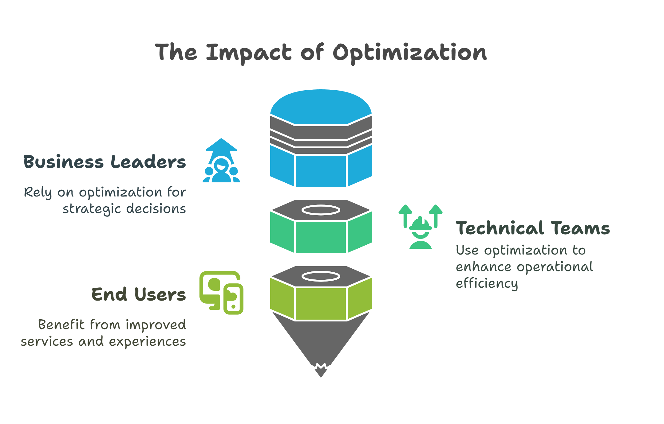
Optimization touches a wide range of stakeholders. Business leaders depend on it for strategic decision-making. Technical teams use it to drive operational efficiency. End users benefit from smoother services, faster responses, and better experiences. Across all levels, better optimization leads to better outcomes.

This post introduces the concept of Learning to Optimize, which is a powerful new approach that combines machine learning with traditional optimization. We’ll explore what Learning to Optimize means, why it matters, and when to use it. To make things concrete, we’ll walk through a real-world example: using deep learning to optimize resource allocation in 6G wireless networks.

What is Learning to Optimize?

Learning to Optimize is the process of training a machine learning model to replace or speed up complex optimization tasks. Instead of solving an optimization problem from scratch every time, we “teach” a model how to find good solutions efficiently. The model learns patterns in the problem structure and uses them to make fast, high-quality decisions.

Intuition: Think of it like teaching a chef how to cook a dish without needing to read the recipe every single time. Once the chef has practiced and internalized the best cooking patterns (e.g., the ingredients, techniques, and timing), they can cook efficiently and adapt to slight variations without starting from zero. Similarly, a model that learns to optimize can make decisions quickly and intelligently without re-solving the full problem every time.

What Learning to Optimize is not: It is not simply making a prediction or forecasting an outcome based on raw data, like predicting next month’s sales figures. Rather, it focuses on learning the decision-making process itself, i.e., how to choose actions or allocations that optimize a given objective.

In simple terms, Learning to Optimize means shifting from repeatedly solving complex problems manually to creating a model that knows how to solve them automatically. It allows businesses to make better decisions faster, at scale, and with lower computational costs.

Real examples:

• In logistics, instead of recalculating the best delivery routes each day with a traditional solver, a model trained through Learning to Optimize can instantly suggest near-optimal routes based on real-time traffic data.
• In finance, instead of running complex portfolio optimization programs overnight, a trained model can quickly recommend asset allocations that maximize returns within risk constraints.
• In wireless networks, Learning to Optimize can allocate frequencies and power levels dynamically, enabling faster and more efficient communication without manually solving optimization problems each time.

Why is Learning to Optimize Important?

Learning to Optimize offers powerful business impacts that can redefine how organizations operate. One of its most significant benefits is the dramatic acceleration of decision-making processes. Traditional optimization methods often require solving complex problems from scratch, which can be time-consuming and computationally expensive. By contrast, a model trained to optimize can deliver near-instantaneous decisions, allowing businesses to respond quickly to changing conditions.

This ability to make real-time decisions is crucial for applications such as traffic control, dynamic pricing, and network optimization. When systems need to adapt immediately to new data or unexpected events, waiting for lengthy optimization computations is simply not an option. Learning to Optimize enables real-time operations, making businesses more agile and resilient.

Additionally, Learning to Optimize significantly cuts computation costs. Running complex solvers repeatedly can be expensive, both in terms of hardware and energy consumption. A learned model, once trained, can perform inference with minimal computational resources, leading to substantial cost savings over time.

Companies that master Learning to Optimize gain a strong competitive advantage. They can move faster, make smarter decisions, and operate more efficiently than competitors who rely on traditional methods. In highly competitive industries, the ability to optimize operations in real time can be the difference between leading the market and falling behind.

Key Steps of a Learning-to-Optimize Framework

A Learning-to-Optimize framework follows a structured process to ensure that the machine learning model can effectively replace or accelerate the optimization solver. Below are the detailed steps:

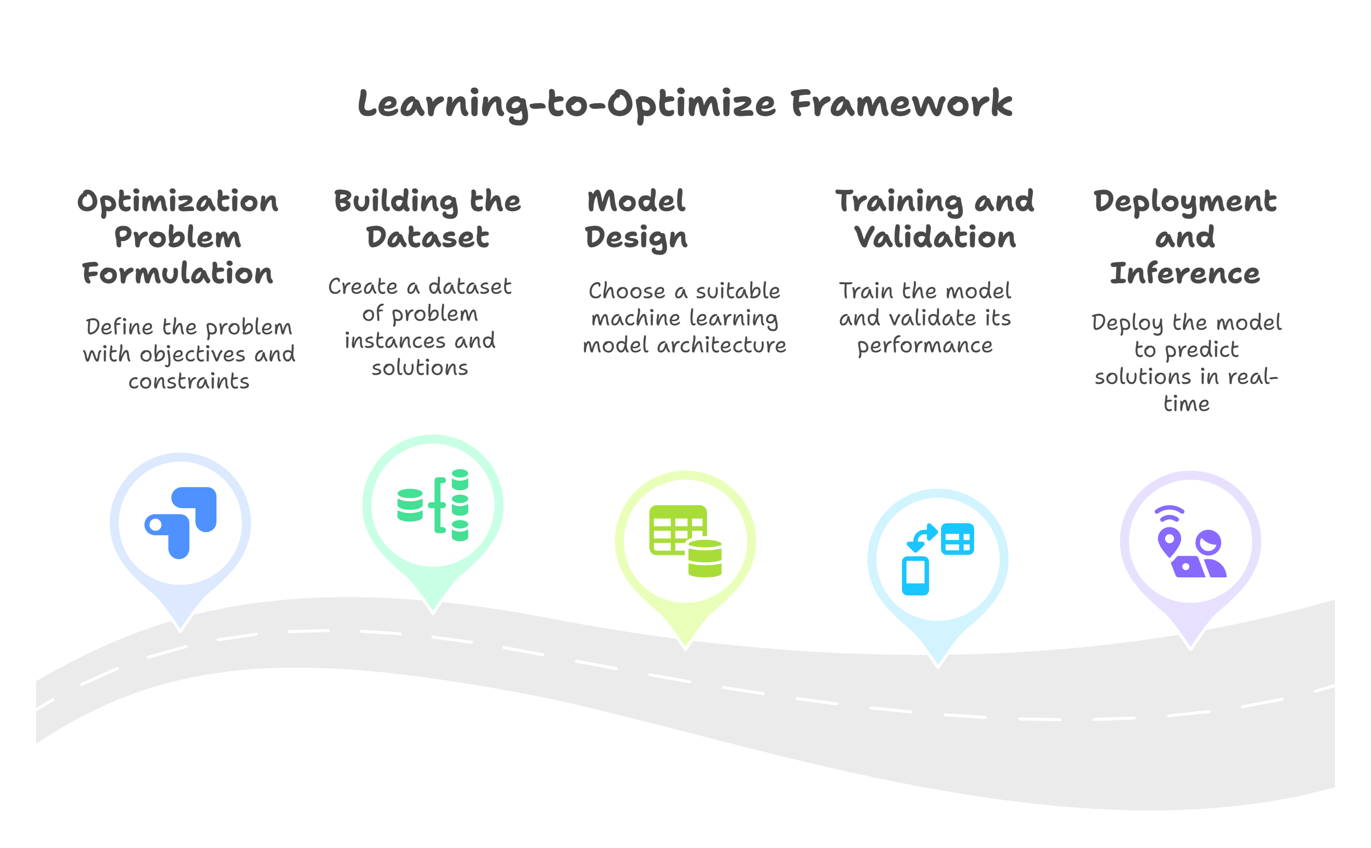
1. Optimization Problem Formulation

The first and most critical step is to clearly define the original optimization problem. This requires a solid foundation in optimization theory, operations research, and domain-specific knowledge. The formulation must accurately capture the objectives, constraints, and operational realities of the problem.

For example, in supply chain management, the goal might be to minimize total delivery time while respecting constraints like vehicle capacity limits, delivery time windows, and traffic conditions. A poor formulation can lead to models that optimize the wrong objective or violate critical real-world constraints, such as delivering goods late or overloading vehicles.

2. Building the Learning-to-Optimize Dataset

Once the problem is formulated, the next step is to build a dataset containing examples of problem instances and their corresponding solutions. The quality of the dataset directly impacts the model’s performance. Ideally, this dataset consists of globally optimal solutions. However, for many complex optimization problems, finding global optima is computationally infeasible. In these cases, high-quality locally optimal solutions or feasible solutions that significantly outperform naive approaches are used.

For example, in nonconvex mixed-integer optimization problems, heuristic or approximate algorithms can generate sufficiently good solutions for training.

3. Model Design: Learning the Mapping

The core of the framework is building a machine learning model that learns the mapping from input features (problem parameters) to optimal decisions.

Depending on the problem structure, convolutional neural networks (CNNs), graph neural networks (GNNs), or other architectures might be chosen to exploit specific patterns, spatial structures, or relational information.

4. Training, Validation, and Testing

The model must be trained on the dataset with careful validation to avoid overfitting and to ensure generalization to unseen instances.

Evaluation metrics are chosen based on how well the model approximates the true optimization solutions while respecting constraints. Testing on out-of-sample data verifies the model’s practical utility.

5. Deployment and Inference

Finally, the trained model is deployed to predict optimized solutions for new problem instances in real time. Compared to solving each instance with a traditional solver, inference through the trained model offers significant speedups and computational savings.

Importantly, a Learning-to-Optimize framework requires human-in-the-loop involvement. Human expertise is crucial for both formulating the optimization problem correctly and building a high-quality solution dataset. Without domain knowledge and careful problem structuring, the model risks learning shortcuts that do not align with the real-world goals or constraints of the system.

When to Use Learning to Optimize?

Learning to Optimize is most valuable in situations where traditional optimization methods struggle to keep up with the demands of the system. If solving the optimization problem from scratch is too slow, too complex, or too costly to do frequently, it may be a strong candidate for a learning-to-optimize approach. For example, large-scale scheduling, resource allocation, or supply chain management problems often fall into this category.

Another key scenario is when systems require real-time decision-making. In areas like autonomous driving, online recommendations, or dynamic network management, the environment can change rapidly, and decisions must be made immediately. Traditional solvers are often too slow for these use cases, whereas a trained model can make quick, approximate decisions that are good enough to meet operational needs.

Finally, Learning to Optimize is most effective when the underlying structure of the optimization problem remains relatively stable over time. If the patterns and relationships in the data do not change dramatically, a model trained once can continue to perform well across many different instances, saving time and computational resources compared to re-solving the optimization anew each time.

Why Learning to Optimize is Still Needed Even with Machine Learning and LLMs

While machine learning models and large language models (LLMs) like ChatGPT, Claude, Grok, or Gemini have revolutionized many aspects of technology and decision-making, they are not always efficient at solving constrained optimization problems. For example, although LLMs can provide suggestions or approximate solutions, they are not designed to find precise, feasible solutions to problems that require strict adherence to mathematical constraints, such as those found in logistics planning or network resource allocation.

Constrained optimization problems typically need to be formulated mathematically and solved using specialized algorithms to ensure feasibility and optimality. While LLMs can assist in formulating these problems or suggesting approaches, the real challenge lies in solving them quickly and effectively. For standard problems like linear programming or convex optimization, it is possible for LLMs to call existing optimization solvers. However, the computational cost and solving time become significant as the problem size grows, especially when solutions are needed frequently or in real time.

Moreover, for complex problems with intricate constraints—such as nonconvex mixed-integer problems—LLMs often struggle to produce high-quality solutions. Their outputs may be infeasible, suboptimal, or computationally inefficient. In contrast, Learning to Optimize focuses specifically on training models that can generate solutions efficiently and effectively, making it a critical tool when fast, reliable decision-making is needed in complex, constraint-heavy environments.

Detailed Example: Learning to Optimize 6G Network Resource Allocation

Overview of 6G Technology and Problem Motivation

What is CFmMIMO and Why Does It Matter?

One of the promising technologies for future 6G wireless networks is called Cell-Free Massive MIMO, or CFmMIMO for short. Instead of using a single tower (or base station) to serve users in a fixed area like we do today, CFmMIMO uses many small access points spread out across a wide area. These access points work together to serve users, no matter where they are, creating a smoother and more consistent connection.

Benefits of CFmMIMO

• Better coverage: Users don’t have to worry about being far from a tower. Multiple access points can work together to serve them.
• Faster data speeds: By combining signals from different points, users can get better performance.
• Lower energy use: Because signals travel shorter distances, less power is needed.
• Less delay: Having access points closer to users reduces the time it takes for data to travel.

Challenges with CFmMIMO

While it sounds great, CFmMIMO isn’t easy to manage. Here are some of the main challenges:

• Limited power: Each access point has a small power limit, so users have to share that power.
• Signal interference: If not managed carefully, signals meant for one user might interfere with others.
• Limited data links: The connection between access points and the main network can only handle so much data.
• Minimum service requirements: Every user expects a basic level of service, and we have to make sure they get it.
• Access point limits: Each access point can only serve a few users at once due to equipment limits.

Why User Association and Power Control Are Important

Wireless systems are complex because the environment is always changing. Signals can get weaker, bounce off buildings, or interfere with each other. Two of the most important decisions we need to make are:

• Which access point should serve which user? (This is called user association.)
• How much power should each access point use for each user? (This is called power control.)

If we make smart choices for these two things, we can make sure everyone gets good service while using the least amount of energy and avoiding interference.

Business Impact

If we can solve these challenges, 6G networks will be faster, more reliable, and cheaper to run. This is good news for:

• Telecom operators, who can serve more users with fewer resources.
• Equipment providers, who can build smarter, more efficient systems.
• Cloud providers, who might help process the data involved.
• Everyday users, who will get better service.

The Optimization Problem

To make all this work, we need to solve a math problem. The goal is to get the highest possible performance across the network (called spectral efficiency) while following all the rules and limits:

• Each access point can’t use more than a certain amount of power.
• The data connection to each access point can only carry so much.
• Every user should get a fair minimum amount of service.
• Each access point can only serve a certain number of users.

What Is Spectral Efficiency?

Spectral efficiency (SE) is just a fancy way of asking: “How much data can we send using a limited amount of bandwidth?” Imagine two highways with the same number of lanes. The one that moves more cars per hour is more efficient. In our case, the cars are data.

A Simple Version of the Problem

We want to maximize the total SE of all UEs in the network.

\[\max_{\{a_{mk}\}, \{p_{mk}\}} \sum_{k=1}^K R_k (\{a_{mk}\}, \{p_{mk}\})\]

where \(R_k\) is the SE received by user \(k\).

Variables:

• User Association: A binary variable \(a_{mk}\) where \(a_{mk} = 1\) if AP \(m\) serves UE \(k\), 0 otherwise.
• Power Allocation: continuous variable \(p_{mk}\) is the power allocated by AP \(m\) to UE \(k\).

Here, \(R_k\) is a complex logarithmic function that reflects how the wireless environment behaves. It depends on factors like signal strength and interference. The decision of which access points serve which users (\(a_{mk}\)) and how much power is allocated (\(p_{mk}\)) will affect signal strength and interference, leading to the change in \(R_k\).

In both theory and practice, \(R_k\) depends explicitly on user association and power control decisions. Theoretically, this relationship is modeled using clean, idealized formulas based on Shannon’s theory, signal power, and interference. In practice, however, real-world imperfections such as hardware limits and unpredictable interference make modeling the function \(R_k\) more complex.

Simplified Constraints:

• \(\sum_{k} p_{mk} \leq P_m^{\text{max}}\) (Transmit power limit per AP)
• \(\sum_{k} R_k \leq C_m^{\text{backhaul}}\) (Backhaul capacity limit per AP)
• \(R_k \geq R_k^{\text{target}}\) (Minimum data rate per UE)
• \(\sum_{k} a_{mk} \leq N_m^{\text{max}}\) (Max number of UEs served per AP)

which mean:

• Each access point stays within its power limit.
• Each access point doesn’t exceed its data link capacity.
• Each user gets at least their minimum service.
• Each access point serves only a limited number of users.

This optimization problem is inherently a mixed-integer nonconvex problem, making it extremely challenging to solve quickly in large-scale 6G networks, which is why Learning to Optimize becomes crucial.

Since this post focuses on the overall concept rather than solving the problem step-by-step, we will skip the detailed mathematical formulation.

Solving the Optimization Problem

To solve the complex optimization problem of user association and power control, we use a method called Successive Convex Approximation (SCA).

What is SCA?

SCA is an advanced technique for solving problems that are too complicated to tackle all at once. Many real-world optimization problems are “non-convex”, meaning they have lots of hills and valleys, making it hard to find the very best solution. Instead of trying to solve the messy problem directly, SCA works step-by-step:

• At each step, it approximates the difficult problem with a simpler, easier (convex) problem.
• It solves this simpler version to get a better guess.
• Then it updates the problem based on this new guess and repeats the process.

Intuition: Think of it like climbing a foggy mountain. Instead of trying to find the highest peak right away, you look around your immediate area, climb to the highest nearby point you can see, and then reassess from there. Step by step, you get closer to the top.

When we use SCA, the solution we find satisfies a necessary condition for being a global best solution. One type of this condition is called the Fritz John condition (named after the mathematician Fritz John).

It means the solution we find is at least a “smart” point—not just some random guess. It’s like reaching a point on the mountain where you can’t immediately find any nearby path that goes uphill. You might not be at the tallest mountain peak in the entire region, but you are somewhere meaningful and high up.

While SCA doesn’t guarantee the absolutely highest peak (global optimum) in all cases, it does ensure that we’ve reached a point that makes sense mathematically and practically.

How to Handle Binary Variables

In the original problem formulation, user association variables are constrained to be binary (i.e., an access point either serves a user or it doesn’t). However, directly optimizing over binary variables makes the problem combinatorial and non-convex.

To address this, we relax the binary constraint by reformulating it into two equivalent continuous constraints. These constraints are then incorporated into the objective function using a penalty method. This allows the optimization to proceed in the continuous domain, which is compatible with the SCA framework.

By tuning the penalty parameters properly, the SCA algorithm converges to solutions that closely satisfy the original binary constraints, resulting in user association variables that are exactly binary or extremely close (within a very small error margin).

Intuition: Instead of forcing hard binary decisions during optimization, we let the model explore continuous values but penalize it for straying too far from 0 or 1. Over time, the optimization “learns” to favor clean binary-like decisions naturally, much like softly guiding a student to either fully commit or fully avoid a choice, rather than staying indecisive.

Why SCA and penalty-based reformulations?

Other methods like exhaustive search and mixed-integer programming are too slow or intractable even for small-scale networks. Heuristic and greedy methods are fast but often yield poor-quality or infeasible solutions. In contrast, SCA with penalty-based reformulations efficiently handles non-convexity and binary constraints, offering high-quality solutions with theoretical convergence. SCA strikes the right balance: it’s efficient, scalable, and principled, making it well-suited for joint user association and power control problems.

Building the Learning-to-Optimize Dataset

To train a machine learning model to make smart decisions in wireless networks, we first need to build a dataset.

Exploratory Data Analysis (EDA) and Feature Engineering

We simulated different network setups by randomly placing Access Points (APs) and Users (UEs). This helps reflect real-world conditions, where UEs move around and the network changes.

Next, we measured how strong or weak the signals are between each AP and each UE. This is captured by what’s called a large-scale fading coefficient. It tells us how much the signal weakens as it travels due to distance or things like buildings and walls. Signals are stronger when UEs are close to an AP, and weaker when they’re farther away.

This is important because a UE’s large-scale fading coefficient (based on location) directly influences both UE association and power control decisions. A UE closer to an AP is more likely to be selected by that AP for service because the connection requires less transmission power and results in better signal quality. On the other hand, UEs farther from an AP may require more power to maintain a reliable connection. Since each AP has a limited power budget, serving distant UEs is more costly and might not be efficient. Therefore, the model must learn to balance UE association and power allocation based on spatial relationships between UEs and APs.

We chose to use only this type of signal information (large-scale fading) as input to the model. While other types of signal changes (like small-scale fading or quick fluctuations due to movement or interference) exist, they change too fast and are hard to track in real time. Large-scale fading changes slowly and is more reliable for decision-making.

What the Dataset Looks Like

For each network setup, the dataset includes:

• Input: Large-scale fading coefficients between each AP and each UE.
• Target output: The best way to connect UEs to APs and assign power, based on a strong optimization method.

Building the Dataset

To figure out what the best decisions look like, we used an optimization method Successive Convex Approximation (SCA). For each setup, SCA calculated:

• Which AP should serve which UE.
• How much power each AP should use for each UE.

These results became the answers our model should learn from. Once trained, the model can make similar high-quality decisions instantly, without having to run the slow optimization process every time.

This dataset will teaches a model how to make smart network decisions by learning from examples where the best possible choices are already known.

Model Development

To make fast, smart decisions in a wireless network, we built a machine learning model based on a Convolutional Neural Network (CNN). The goal of the model is to learn from our dataset how to choose the best way to connect users to access points and how to assign transmission power in each scenario.

Why We Chose a CNN

We specifically chose a CNN instead of other types of neural networks for several important reasons:

• Preserving spatial structure: The problem has an inherent spatial structure (access points and users are laid out in space), and CNNs are excellent at capturing local patterns like strong signals or interference.
• Efficiency: CNNs use a small number of parameters compared to fully connected networks. This reduces the risk of overfitting and speeds up training.
• Scalability: Because CNNs work locally (only looking at neighboring points at a time), they scale better when the number of APs and UEs grows.
• Generalization: CNNs generalize better to unseen network layouts because they focus on local relationships rather than memorizing global structures.

CNN Workflow and Design

For this example, we use normalized power (\(P_m^{\max} = 1, \forall m\)).

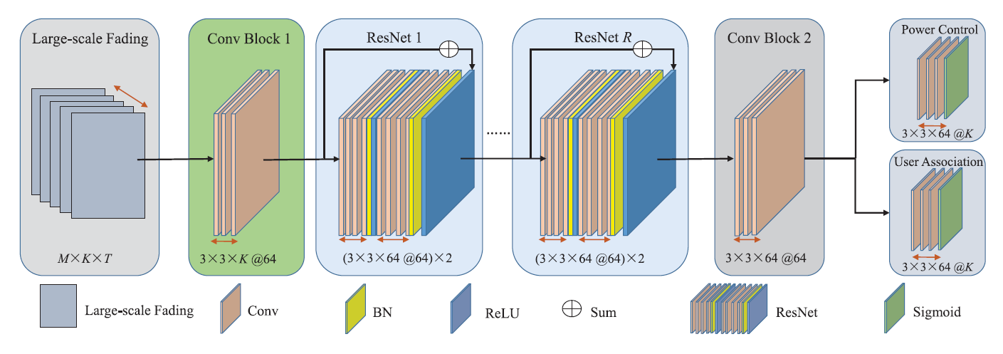
The CNN model architecture is carefully designed based on the following components:

Input Layer

• Input: A large-scale fading matrix showing signal strength between APs and UEs.
• Size: M x K (M = number of APs, K = number of UEs).
• Number of training samples: T

Conv Block 1

• A 2D convolution layer with 64 3×3 filters, giving 64 output learned features (e.g., signal strength patterns, interference cues, proximity effects, context from neighboring APs or UEs, and etc)
• Each filter has weights that are learned during training.
• Purpose: Extract local features for AP-UE pairs.
• How it interacts with the input: In Conv Block 1, each 3×3 filter slides across the input matrix (which represents AP–UE relationships), examining a small local patch one step at a time. At each position (corresponding to one AP–UE pair), the filter looks at a 3×3 neighborhood, multiplies each input value by its corresponding filter weight, sums them up, and produces one single output feature for that AP–UE pair. Since there are 64 different filters, each AP–UE pair ends up having 64 output features — one feature from each filter — capturing different learned features.
• Why 3×3? A small window captures local dependencies without overwhelming complexity.
• Why 64 output learned features? Enough capacity to learn a wide range of basic features.
• Output size: M x K x 64.
• Intuition: The filter acts like a magnifying glass. It scans small local regions of the input. It extracts important local features like “strong connection here,” “weak connection there,” etc.

Residual Blocks (ResNet-R)

• R residual blocks, each containing two convolutional layers.
• Each convolutional layer uses 3×3 filters across 64 channels, maintaining the feature depth.
• Batch Normalization is applied after each convolution to stabilize training by normalizing the feature distributions, speeding up convergence and allowing higher learning rates.
• ReLU activation is applied after Batch Normalization to introduce non-linearity, enabling the network to learn complex, non-linear mappings and preventing vanishing gradients.
• Skip connections are added to each block, allowing the input to be directly added to the output. This helps gradients flow more easily during backpropagation, solving the vanishing gradient problem and enabling much deeper networks to be trained effectively. Skip connections also help the network remember the input, allowing it to preserve important information and only learn the differences (residuals) needed to improve the mapping.
• Purpose: Deepen the network to learn complex hierarchical features, where deeper layers extract more abstract patterns based on local relationships.
• Intuition: Normal networks try to learn everything from scratch at every layer. ResNet helps networks learn better by making layers focus only on small improvements from Conv Block 1, not full transformations — while remembering and preserving the good parts of the input through skip connections. Like climbing a mountain. Instead of jumping to random new points, you step slightly up from where you already are.

Conv Block 2

• A 2D convolution layer with 3×3 filters, operating on the 64 feature maps produced by the previous layers.
• Purpose: Refine and unify the deep features extracted by the ResNet blocks.
• Why 3×3? Maintains local spatial relationships while slightly adjusting and smoothing the features before output.
• This layer aggregates the various complex patterns detected by earlier layers into a more consistent, task-friendly representation.
• It prepares a clean and focused feature map that contains distilled information needed for the final predictions made by the output heads.
• Intuition: Like as a final adjustment layer to align the network’s learned features with the specific needs of power control and user association prediction.
• Output size: M x K x 64.

After Conv Block 2, the network splits into two branches of output heads:

Power Control Head

• A specialized output branch designed to predict normalized power allocation decisions for each AP-UE pair.
• Structure: A 2D convolution layer with 3×3 filters, followed by a sigmoid activation function.
• Why Conv? Using a convolutional layer ensures that local spatial patterns and relationships between neighboring APs and UEs are preserved during the final prediction. This helps the model make decisions that are sensitive to nearby network conditions.
• Why 3×3? A small receptive field captures local dependencies without blending unrelated distant AP-UE interactions.
• The 3×3×64 kernel collects information from a local 3×3 neighborhood across all 64 learned features, multiplies and sums them, and produces one output number at each AP-UE pair.
• The sigmoid activation constrains the output values between 0 and 1, matching the normalized power control targets used during training. This guarantees that the model outputs physically meaningful power allocations suitable for real-world system constraints.
• Output: A matrix of size M x K, where each element represents the predicted normalized power for a specific AP-UE pair.

User Association Head

• Conv layer (3×3, 64 filters) followed by sigmoid activation, which is similar to Power Control Head
• Output: A matrix of size M x K, where each element represents an association probability (range 0 to 1) for each AP-UE pair.

Even though the Power Control Head and User Association Head have the same structure (3×3×64 convolution + sigmoid), they predict different types of outputs because they are trained with different ground truth labels (continuous power vs. binary association).

Note that standard practice in CNNs — especially with 3×3 convolutions — involves applying padding of 1 pixel on all sides. This preserves the spatial size of the input, ensuring that the Access Point–User Equipment (AP–UE) relationship grid (M × K) remains consistent throughout the network. Padding is thus implicitly applied in ConvBlock 1, the ResNet blocks, and ConvBlock 2. Also, the bias term from each layer is omitted here to ensure clarity expression.

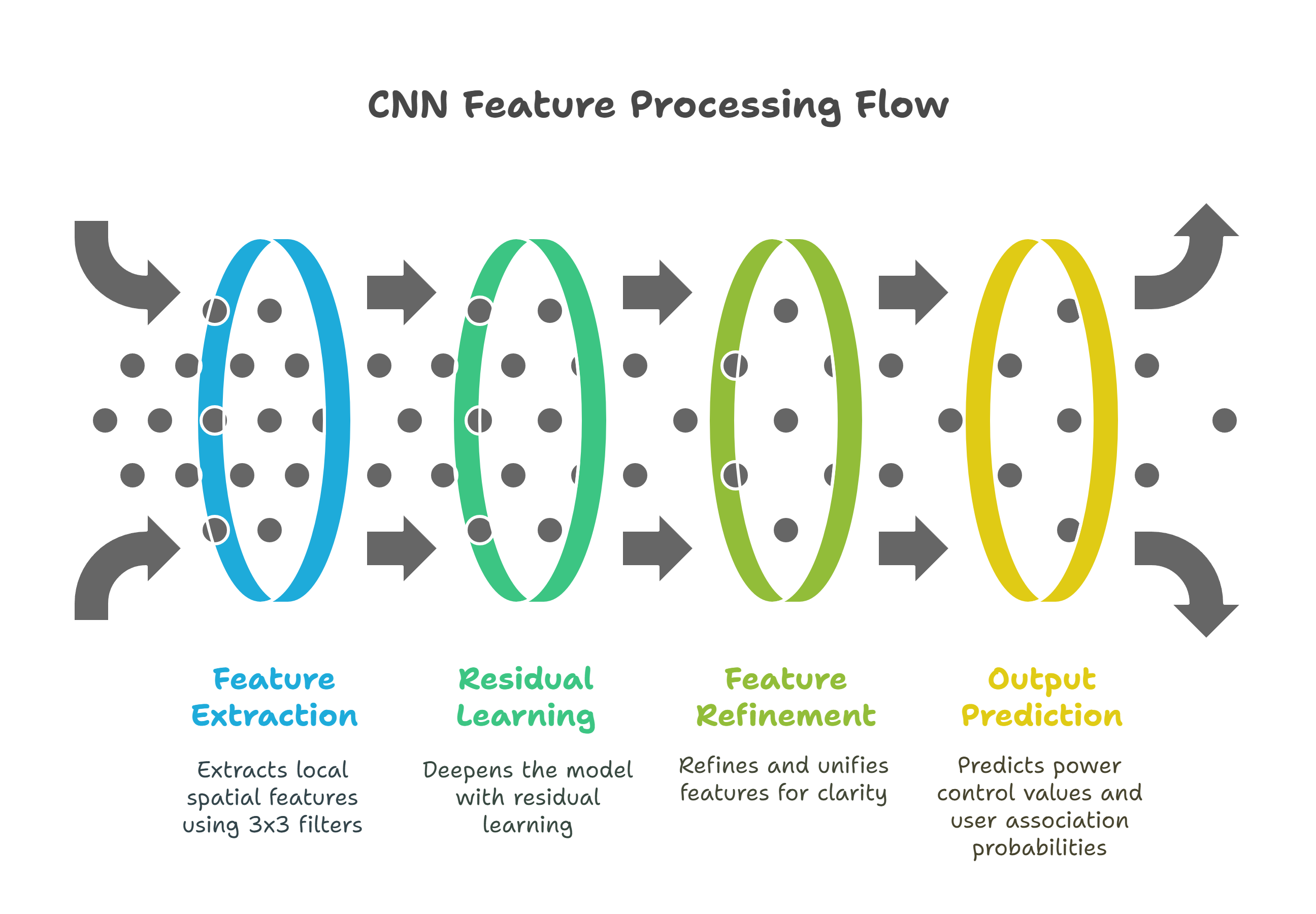
Summarized CNN Workflow

The CNN begins with Conv Block 1, which extracts local spatial features from the large-scale fading matrix of AP-UE pairs using 3×3 filters, turning each AP–UE pair into a 64-dimensional feature vector. This is followed by ResNet blocks, which deepen the model with residual learning, allowing it to learn increasingly complex patterns while preserving input information through skip connections. Conv Block 2 then refines and unifies these features, preparing a clean, task-ready representation. Finally, the network splits into two Output Heads: one predicts normalized power control values and the other predicts user association probabilities, to produce interpretable outputs for every AP–UE pair.

Why Not Fully Connected Networks?

We considered using fully connected networks but rejected them for several reasons:

• Too many parameters: Fully connected layers grow dramatically in size as M and K increase.
• Loss of spatial structure: Fully connected layers ignore the natural 2D structure between APs and UEs.
• Higher overfitting risk: Fully connected networks tend to memorize training data rather than generalize.

Model Training

To train the proposed CNN model, we follow the supervised learning approach with 28000 input samples.

The model is trained to minimize the Mean Squared Error (MSE) between its predicted outputs and the SCA-generated ground truths, separately for both power control and user association. The final loss is the average of both components, ensuring equal emphasis on both tasks. Mathematically, the loss is minimized over training batches of size of 512, and the MSE is averaged across all samples in each batch. The MSE metric is chosen for its simplicity and effectiveness in penalizing large deviations while encouraging the model to approximate decisions closely.

Training was carried out using the Adam optimizer and maximum 400 epochs. All experiments and model training were implemented in MATLAB, utilizing its deep learning toolbox for defining the CNN architecture, training loops, and performance evaluation.

The model’s architecture was tuned by varying the number of ResNet blocks, filter sizes, and activation functions to achieve the desired training accuracy. Performance was validated by monitoring both training and validation loss curves, which showed consistent convergence and minimal overfitting.

A training epoch refers to one complete pass through the entire training dataset during model training. In each epoch, the dataset is divided into mini-batches. For each batch, the model makes predictions, computes the error (loss), and updates its weights through backpropagation. Multiple epochs are needed because a single pass is usually not enough for the model to learn meaningful patterns. Repeated passes allow the model to gradually improve. For example, if your dataset has 10,000 samples and the batch size is 512, each epoch processes all 10,000 samples once across multiple iterations. Training typically runs for tens or hundreds of epochs until the model converges. Think of it like studying: one epoch is like reading the full textbook once, while multiple epochs are like reviewing it several times to reinforce understanding.

The Adam optimizer (Adaptive Moment Estimation) is a widely used algorithm for training neural networks that combines the strengths of two other methods: momentum and adaptive learning rates. It adjusts the learning rate for each model parameter individually by using both the average of past gradients (direction) and the average of their squared values (size). This allows it to make stable, efficient updates even when gradients vary in scale. The Adam optimizer works like a smart GPS for training a neural network: it remembers the direction it’s been going (momentum) and adjusts its speed (learning rate) based on how bumpy the path is. This helps the model take smoother, faster, and more accurate steps toward better performance without overshooting or getting stuck.

We choose Adam optimizer because it typically converges faster than traditional methods like stochastic gradient descent, making it especially suitable for training deep models such as CNNs.

Post-Processing Procedure: Ensuring Feasible Solution

To ensure the CNN outputs remain feasible with respect to system constraints, the paper applies a lightweight two-step post-processing procedure:

• If any AP’s predicted transmit power exceeds its allowed maximum, all its power control values are proportionally rescaled to satisfy the constraint.
• After recalculating the spectral efficiencies, if any AP exceeds its fronthaul capacity, all user spectral efficiencies are scaled down to ensure no AP is overloaded.

These are the constraints that are most likely to be violated.

This approach guarantees that the final solution respects power and fronthaul constraints without retraining the model, allowing for fast, constraint-compliant inference in real time.

Model Evaluation

The performance of the proposed CNN model was evaluated by comparing its outputs to the optimal solutions obtained from the SCA algorithm. The key metric used is sum spectral efficiency, which reflects how efficiently the network uses its available resources.

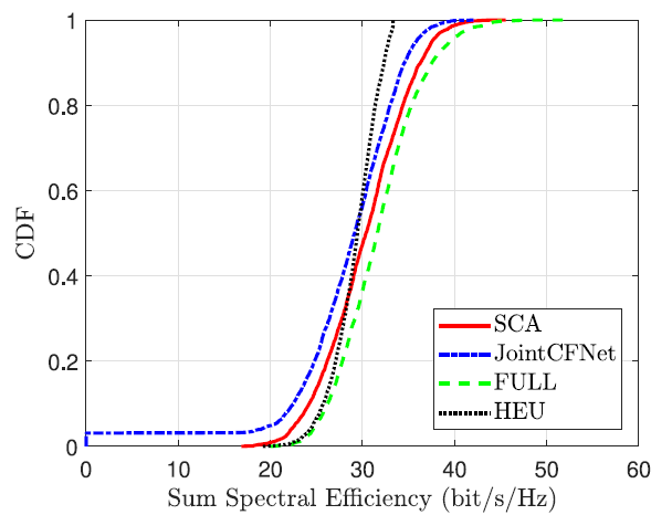
This plot shows the Cumulative Distribution Function (CDF) of the sum spectral efficiency (in bits/s/Hz) for different methods under evaluation.

• X-axis (Sum Spectral Efficiency): Measures the total data rate achieved by all users, normalized by bandwidth. Higher values mean more efficient spectrum usage.
• Y-axis (CDF): For each x-value, it shows the percentage of network realizations where the spectral efficiency was less than or equal to that value.
• Red Curve: SCA (Benchmark Optimal Solution)
• Blue Curve: Proposed CNN Model
• The green and black curves are ignored since they are out of scope of this post.

This plot show that the CNN model achieves over 97% of the spectral efficiency compared to the traditional SCA-based optimization with up to 95% feasible solution. This demonstrating that the model learns to approximate high-quality solutions very effectively.

In addition to accuracy, inference speed was a major focus of evaluation. While the SCA algorithm takes approximately 20 seconds to solve a single instance of the optimization problem, the trained CNN model generates predictions in about 2 millisecond, leading to a speedup of over 1,000×. This dramatic reduction in runtime makes the approach well-suited for real-time deployment, where rapid decision-making is critical — such as in dense 6G wireless networks with dynamic user movement and varying network loads.

These results confirm that the model offers a strong balance between solution quality and computational efficiency, enabling high-performance decisions without relying on slow optimization solvers.

Next Steps for Improvement

While the current model demonstrates high accuracy and efficiency, several enhancements can be explored to further improve its robustness and scalability.

• The training data used in this example is based on static network snapshots. In practice, user positions, channel conditions, and interference patterns can change rapidly. Incorporating dynamic network conditions, such as user mobility, time-varying fading, or variable user traffic demands, into the training data would allow the model to better generalize to real-world deployment scenarios and maintain performance in evolving environments.

• As the network size grows, the current CNN architecture may face challenges in capturing long-range dependencies or efficiently scaling to very large AP–UE grids. To address this, future work could explore Graph Neural Networks (GNNs), which naturally model connectivity, sparsity, and relationships in irregular wireless network topologies. GNNs offer the potential to process large-scale networks more flexibly by learning on graph structures rather than fixed spatial grids.

• The current approach is supervised and learns from offline optimization solutions. Incorporating reinforcement learning (RL) could further enhance the model’s adaptability by enabling it to interact with the environment and improve through trial-and-error. An RL-based agent could learn to make real-time decisions under uncertainty, adapt to unseen scenarios, and even optimize for long-term performance objectives beyond snapshot efficiency.

These extensions would push the model toward a more autonomous, scalable, and real-world-ready learning-to-optimize framework for next-generation wireless systems.

Conclusion

Learning to Optimize connects the strengths of machine learning and mathematical optimization, creating a powerful framework for solving complex decision-making problems more efficiently and intelligently.

From wireless network resource allocation to supply chain planning, this approach has the potential to reshape how industries design and operate their systems.

As real-world challenges grow in scale and complexity, Learning to Optimize is emerging as a vital skillset that every data scientist and engineer should understand and master.

The detailed example in this post is available in my publication.

For further inquiries or collaboration, please contact me at my email.