Building a Machine Learning Model to Estimate Insurance Premiums

Insurance pricing is a complex process where companies determine premiums based on various risk factors such as age, health, income, claims history, and lifestyle. However, the exact pricing models used by insurers are proprietary, making it difficult for customers and businesses to understand premium calculations.

In this project, we build a machine learning model using EDA, feature engineering, and XGBoost to predict insurance premium amounts. By mimicking the insurer’s pricing strategy, our goal is to uncover key factors affecting premiums and develop a data-driven premium estimation tool.

To run the project, we follow the essential steps of a data science project as follows.

1. Problem Definition and Business Understanding

Insurance companies assess risk factors to price policies, but customers often lack transparency on why they are charged certain premiums. A predictive model can:

• Help customers estimate their premiums based on their profile.
• Allow insurers to optimize pricing and detect anomalies.
• Ensure fairness and regulatory compliance in premium calculations.

Our goal is to predict the insurance premium amount a customer would be charged based on their attributes using machine learning models. The model will identify the most important risk factors and help in estimating premiums for new customers.

2. Dataset Description

The dataset train.csv includes various customer attributes that influence premium pricing. Key features include:

Numerical Features

• Age (Float) – Customer’s age.
• Annual Income (Float) – Earnings per year.
• Health Score (Float) – Health risk indicator.
• Previous Claims (Float) – Number of past claims.
• Vehicle Age (Float) – Age of insured vehicle.
• Credit Score (Float) – Financial risk measure.
• Insurance Duration (Float) – Policy period.

Categorical Features

• Gender (Male/Female)
• Marital Status (Single/Married/Other)
• Education Level (High School, Bachelor’s, Master’s, etc.)
• Occupation (Job type, with significant missing values)
• Smoking Status (Yes/No)
• Exercise Frequency (Regular, Occasional, None)
• Property Type (Owned, Rented)
• Location (Urban, Rural, Suburban)

Target Variable

• Premium Amount (Float) – The insurance premium charged by the insurer.

3. Data Exploration Analysis (EDA)

Load Dataset

# All required libraries are imported here
import pandas as pd
import numpy as np
import matplotlib.pyplot as plt
import seaborn as sns
from sklearn.model_selection import KFold
from sklearn.metrics import mean_squared_log_error
from xgboost import XGBRegressor
import scipy.stats as stats
import math
from scipy.stats import kruskal

# Load Dataset
file_path = "train.csv"  
df = pd.read_csv(file_path)

print(f"Data shape: {df.shape}")
print(df.head())
print(df.info())

Output:

Data shape: (1200000, 21)
   id   Age  Gender  Annual Income Marital Status  Number of Dependents  \
0   0  19.0  Female        10049.0        Married                   1.0   
1   1  39.0  Female        31678.0       Divorced                   3.0   
2   2  23.0    Male        25602.0       Divorced                   3.0   
3   3  21.0    Male       141855.0        Married                   2.0   
4   4  21.0    Male        39651.0         Single                   1.0   

  Education Level     Occupation  Health Score  Location  ... Previous Claims  \
0      Bachelor's  Self-Employed     22.598761     Urban  ...             2.0   
1        Master's            NaN     15.569731     Rural  ...             1.0   
2     High School  Self-Employed     47.177549  Suburban  ...             1.0   
3      Bachelor's            NaN     10.938144     Rural  ...             1.0   
4      Bachelor's  Self-Employed     20.376094     Rural  ...             0.0   

   Vehicle Age  Credit Score  Insurance Duration           Policy Start Date  \
0         17.0         372.0                 5.0  2023-12-23 15:21:39.134960   
1         12.0         694.0                 2.0  2023-06-12 15:21:39.111551   
2         14.0           NaN                 3.0  2023-09-30 15:21:39.221386   
3          0.0         367.0                 1.0  2024-06-12 15:21:39.226954   
4          8.0         598.0                 4.0  2021-12-01 15:21:39.252145   

  Customer Feedback Smoking Status Exercise Frequency Property Type  \
0              Poor             No             Weekly         House   
1           Average            Yes            Monthly         House   
2              Good            Yes             Weekly         House   
3              Poor            Yes              Daily     Apartment   
4              Poor            Yes             Weekly         House   

  Premium Amount  
0         2869.0  
1         1483.0  
2          567.0  
3          765.0  
4         2022.0  

[5 rows x 21 columns]
<class 'pandas.core.frame.DataFrame'>
RangeIndex: 1200000 entries, 0 to 1199999
Data columns (total 21 columns):
 #   Column                Non-Null Count    Dtype  
---  ------                --------------    -----  
 0   id                    1200000 non-null  int64  
 1   Age                   1181295 non-null  float64
 2   Gender                1200000 non-null  object 
 3   Annual Income         1155051 non-null  float64
 4   Marital Status        1181471 non-null  object 
 5   Number of Dependents  1090328 non-null  float64
 6   Education Level       1200000 non-null  object 
 7   Occupation            841925 non-null   object 
 8   Health Score          1125924 non-null  float64
 9   Location              1200000 non-null  object 
 10  Policy Type           1200000 non-null  object 
 11  Previous Claims       835971 non-null   float64
 12  Vehicle Age           1199994 non-null  float64
 13  Credit Score          1062118 non-null  float64
 14  Insurance Duration    1199999 non-null  float64
 15  Policy Start Date     1200000 non-null  object 
 16  Customer Feedback     1122176 non-null  object 
 17  Smoking Status        1200000 non-null  object 
 18  Exercise Frequency    1200000 non-null  object 
 19  Property Type         1200000 non-null  object 
 20  Premium Amount        1200000 non-null  float64
dtypes: float64(9), int64(1), object(11)
memory usage: 192.3+ MB

Key actionable insights:

• The dataset contains approximately 1.2 million rows with several categorical features, many of which have a large number of unique categories (such as Exercise Frequency and Education Level).
• This necessitates careful selection of encoding strategies when using simpler models (e.g., Ridge Regression, Linear Regression, Random Forest), or advanced models (e.g., XGBoost, LightGBM) that can natively handle raw categorical features without manual encoding.
• Machine learning models can’t understand raw date formats like “2023-05-15” of Policy Start Date. They need to be transformed to numerical inputs (floats or integers) to learn patterns.

Check Missing Values

• This step is a mandatory step to understand data health, knowing which features have missing data and how much in percentage.
• The result is useful to decide next steps: Drop columns with too many missing values, or impute (fill) missing values, or leave them alone (if very small), or choose a predictive model that can handle missing values automatically.

# Missing Values Analysis 
print("\nMissing Values:\n")
missing_values = df.isnull().sum()
missing_percentage = (missing_values / len(df)) * 100
missing_df = pd.DataFrame({'Missing Values': missing_values, 'Percentage': missing_percentage})
print(missing_df[missing_df['Missing Values'] > 0].sort_values(by='Percentage', ascending=False))

Output:

                      Missing Values  Percentage
Previous Claims               364029   30.335750
Occupation                    358075   29.839583
Credit Score                  137882   11.490167
Number of Dependents          109672    9.139333
Customer Feedback              77824    6.485333
Health Score                   74076    6.173000
Annual Income                  44949    3.745750
Age                            18705    1.558750
Marital Status                 18529    1.544083
Vehicle Age                        6    0.000500
Insurance Duration                 1    0.000083

Key Actionable Insights:

• There are significant missing values in the dataset.
• This requires a careful, feature-by-feature plan to guess/impute missing values or to use some models (like XGBoost, LightGBM) that can natively handle missing values without needing explicit imputation.

Check the Distribution of Categorical Features

This step helps to:

• Understand category balance (detect if some classes dominate). Rare categories might cause instability during modeling.
• Guide encoding decisions (e.g., one-hot, target encoding).
• Spot data quality issues (e.g., typos, unexpected categories).

# Identify Categorical Features
cat_features = df.select_dtypes(include=["object"]).columns.tolist()

# Remove 'Policy Start Date' if it exists (safe removal)
if "Policy Start Date" in cat_features:
    cat_features.remove("Policy Start Date")

# Calculate number of rows and columns for the subplots
n_cols = 3  # Number of columns
n_rows = math.ceil(len(cat_features) / n_cols)

# Create subplots
fig, axes = plt.subplots(n_rows, n_cols, figsize=(18, n_rows * 5))
axes = axes.flatten()  # Flatten in case of a single row

# Plot each categorical feature
for idx, col in enumerate(cat_features):
    ax = axes[idx]
    sns.countplot(data=df, x=col, ax=ax, order=df[col].value_counts().index)
    ax.set_title(f"Distribution of {col}")
    ax.set_xlabel(col)
    ax.set_ylabel("Count")
    ax.tick_params(axis='x', rotation=45)

# Hide any empty subplots
for i in range(len(cat_features), len(axes)):
    fig.delaxes(axes[i])

plt.tight_layout()
plt.show()

Output:

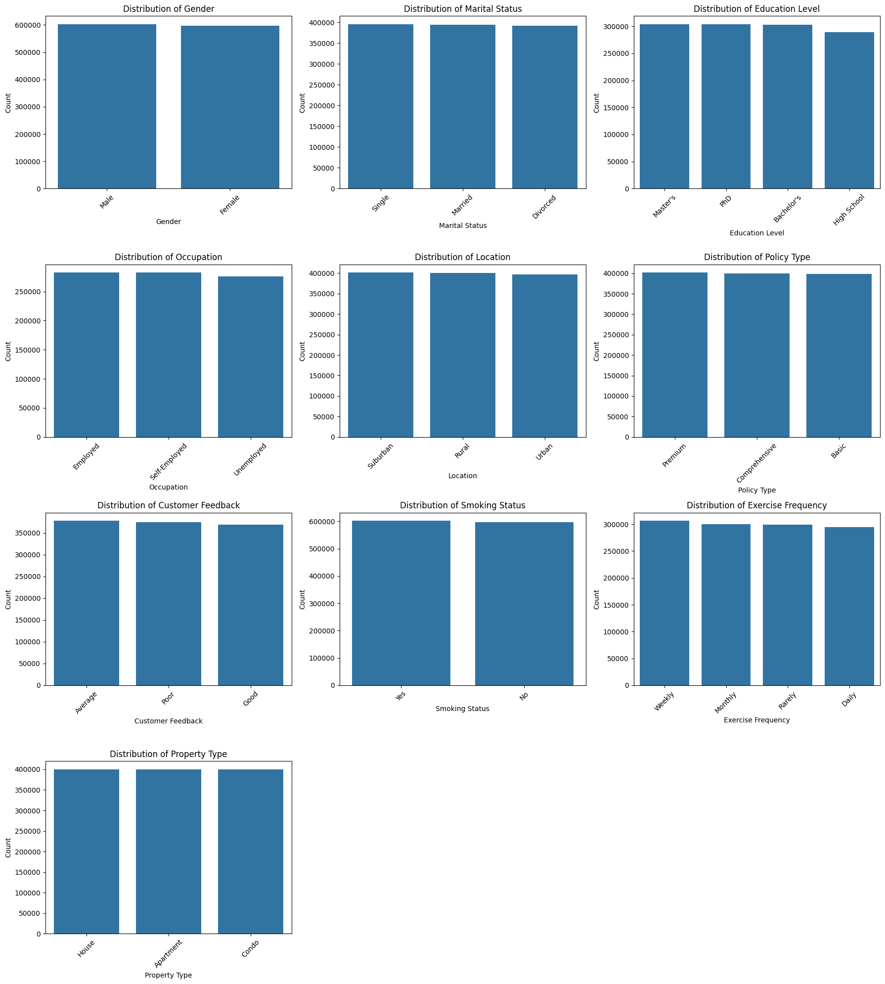
Key actionable insights

• The distributions are balanced overall.
• No major imbalance, so no special resampling (e.g., SMOTE) is needed for these features.
• The categorical features can be safely included in modeling without adjustment.

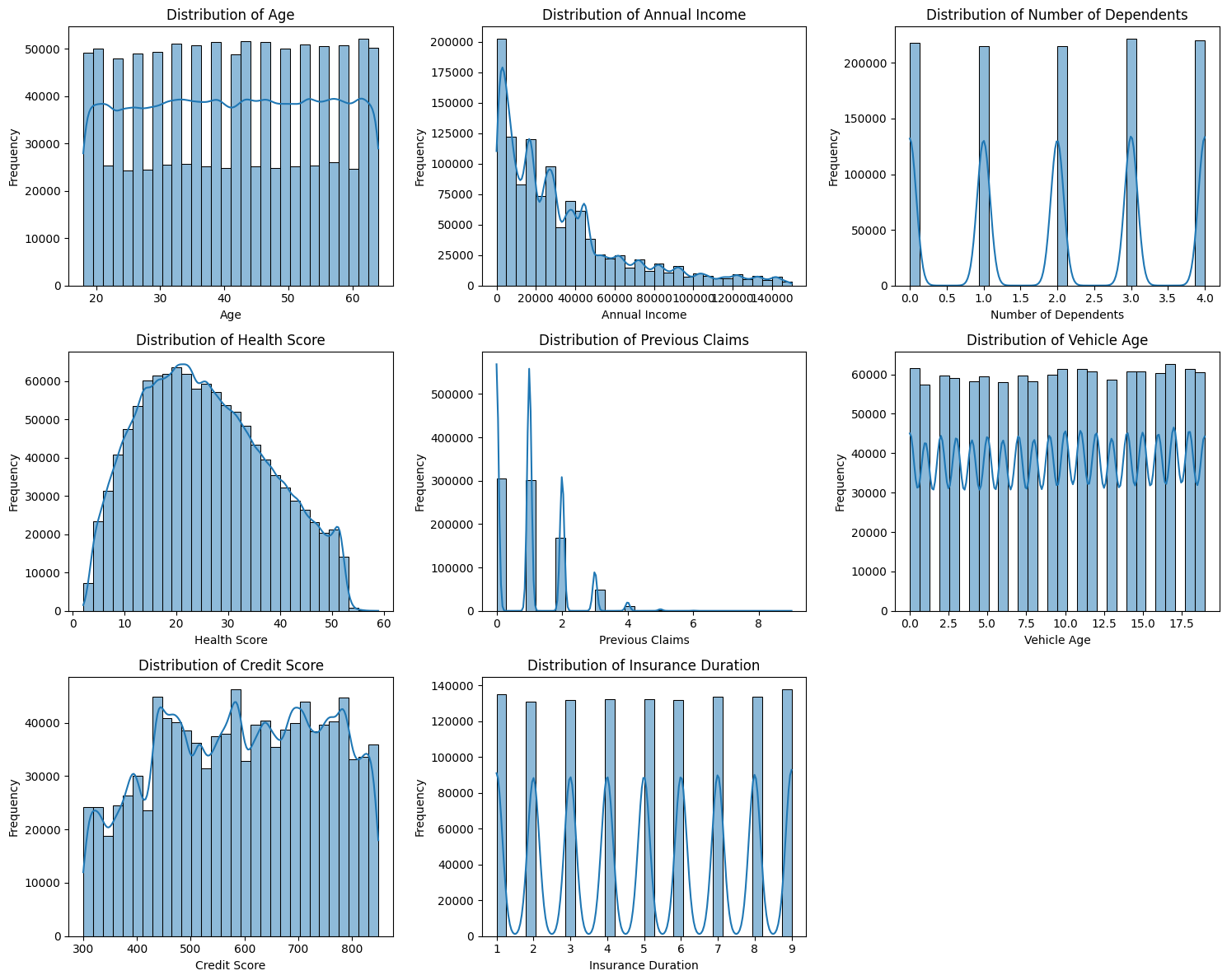
Check the Distribution and Boxplot of Numerical Features

This step helps to:

• Understand the shape of the data (normal, skewed, bimodal, etc.).
• Detect outliers that could affect modeling.
• Decide on transformations or models to handle highly skewed data.
• Identify scaling needs (important for models sensitive to feature magnitudes like Ridge, Lasso).
• Spot data entry errors (e.g., extremely large or negative values where not expected).

# Select Numerical Features
num_features = df.select_dtypes(include=["float64"]).columns.tolist()

# Remove the target if it's in the list
if "Premium Amount" in num_features:
    num_features.remove("Premium Amount")

# Plot all numerical features together
n_cols = 3  # number of columns of plots
n_rows = (len(num_features) + n_cols - 1) // n_cols  # calculate needed rows

plt.figure(figsize=(5 * n_cols, 4 * n_rows))

for idx, col in enumerate(num_features, 1):
    plt.subplot(n_rows, n_cols, idx)
    sns.histplot(df[col], kde=True, bins=30)
    plt.title(f"Distribution of {col}")
    plt.xlabel(col)
    plt.ylabel("Frequency")

plt.tight_layout()
plt.show()

Output:

# Set up the plot grid
n_cols = 3  # Number of columns you want
n_rows = math.ceil(len(num_features) / n_cols)

fig, axes = plt.subplots(n_rows, n_cols, figsize=(18, n_rows * 4))  # Adjust figure size
axes = axes.flatten()

# Plot each numerical feature
for idx, col in enumerate(num_features):
    sns.boxplot(data=df, y=col, ax=axes[idx])
    axes[idx].set_title(f"Boxplot of {col}")

# Hide any empty subplots
for i in range(len(num_features), len(axes)):
    fig.delaxes(axes[i])

plt.tight_layout()
plt.show()

Output:

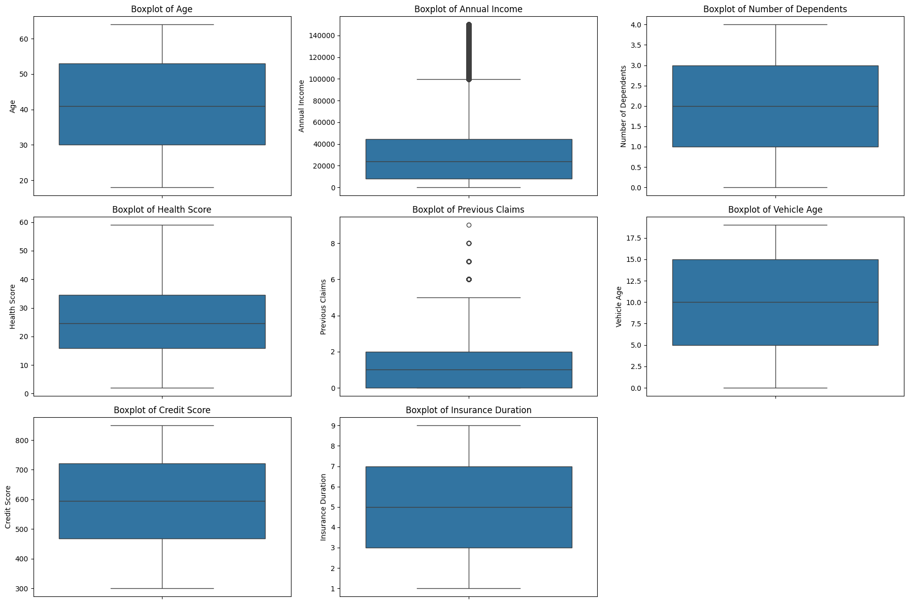
Key actionable insights

• There are a few skewed features and outliers (e.g., Annual Income, Previous Claims). This requires transformation or models (e.g., XGBoost, LightGBM) that can handle skewed numerical features naturally.
• There is no data entry errors (e.g., extremely large or negative values where not expected).
• Previous Claims, Insurance Duration, Number of Dependents are integer with short ranges, representing a meaningful quantity (count, duration, quantity). They are kept as numeric instead of being converted to categorical (e.g., in case of zip code, 1000 and 2000 are categorical).

Check the Distribution and Boxplot of Target Variable (Premium Amount)

Checking the distribution and boxplot protects model performance by exposing skewness and outliers early.

# Distribution of Target Variable (Premium Amount)
plt.figure(figsize=(8, 5))
sns.histplot(df['Premium Amount'], bins=50, kde=True)
plt.title("Distribution of Premium Amount")
plt.xlabel("Premium Amount")
plt.ylabel("Frequency")
plt.show()

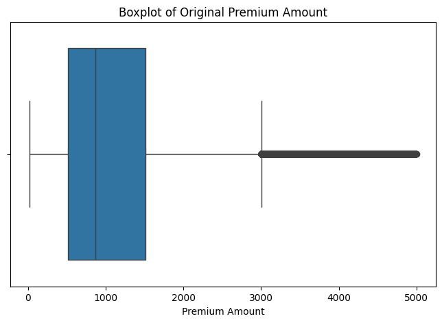
# Boxplot of Original Premium Amount
plt.figure(figsize=(8, 5))
sns.boxplot(x=df["Premium Amount"])
plt.title("Boxplot of Original Premium Amount")
plt.xlabel("Premium Amount")
plt.show()

Output:

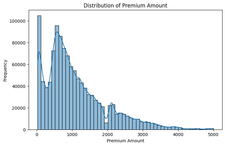
Key Actionable Insights:

• Heavy right skew: Most people have relatively low to moderate premiums, but a small number of people have very large premiums (outliers).
• Outliers are real: There are significant extreme values.
• Wide spread: Premiums vary widely from low to very high, consistent with what we saw in the histogram.
• Log transformation was a good idea: Because it compresses those large premium values and makes the target variable easier for the model to learn.

Check for Multicollinearity Among Numerical Features using a Heatmap

• Multicollinearity happens when two or more features are strongly correlated with each other. For example, “Annual Income” and “Credit Score” might be very correlated — both relate to financial stability.
• If two variables are highly correlated (correlation > 0.8 or < -0.8), they carry redundant information. This can cause problems for some models (especially linear models like Ridge/Lasso).
• This check supports feature engineering decisions. For example, after seeing the heatmap, two highly correlated features might be dropped out, or combined into a new feature, or kept but regularized (e.g., with Ridge Regression).
• The heatmap reveals clusters of correlated variables via colors, finding hidden patterns quickly in data before even fitting a model.

# Correlation Matrix for Numerical Features
numeric_df = df.select_dtypes(include=['number'])

# Compute the correlation matrix
corr_matrix = numeric_df.corr()

# Plot the heatmap
plt.figure(figsize=(12, 8))
sns.heatmap(corr_matrix, annot=True, fmt=".2f", cmap="coolwarm", linewidths=0.5)
plt.title("Correlation Matrix of Numerical Features")
plt.show()

Output:

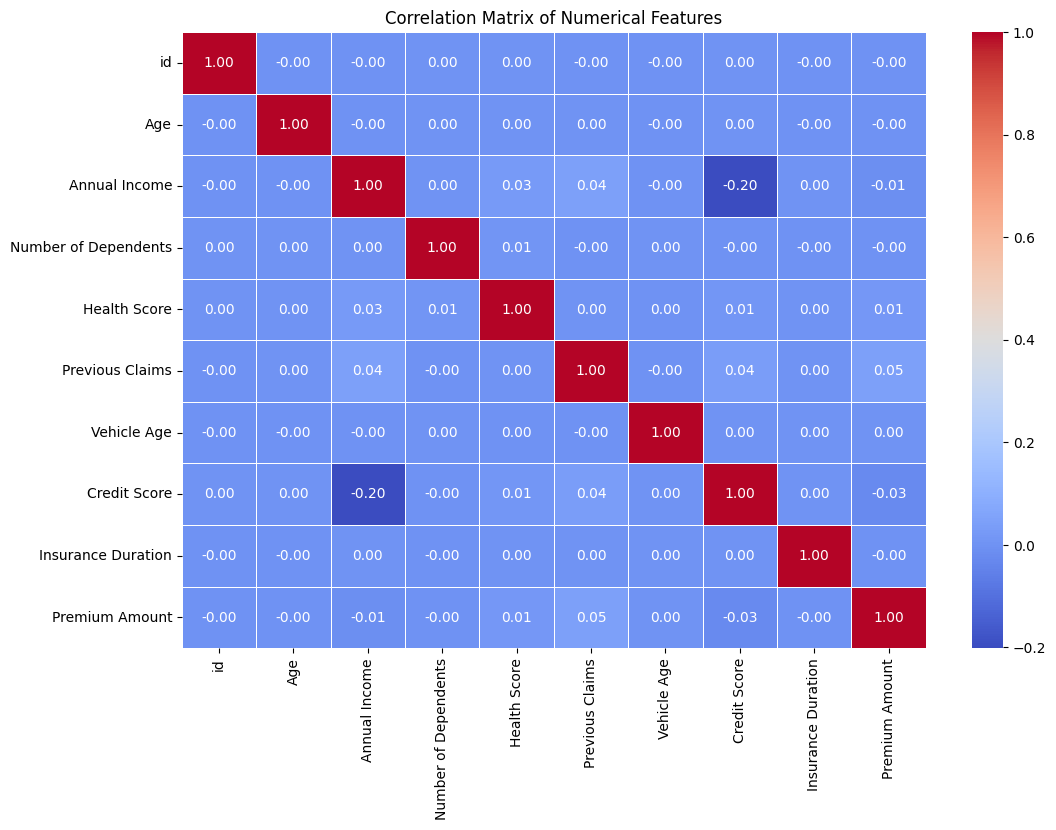
Key Actionable Insights:

• Numerical features show little to no correlation with each other.
• Keep all numerical features for modeling.
• We don’t need to remove or combine features based on correlation.
• Skip dimensionality reduction (e.g., PCA is not needed here).

Check Dependencies between Categorical and Target Features

This step helps to:

• Understand Relationships: Check whether different categorical features (like “Gender”, “Policy Type”, etc.) might make real differences in the target feature (“Premium Amount”).
• Improve Feature Engineering: Strong dependency may suggest we should interact features or create new features.

Since Premium Amount is highly skewed, we use the Kruskal-Wallis H-test to test the dependency between categorical features and Premium Amount (instead of the commonly used ANOVA test with the assumption of normally distributed data).

cat_features = df.select_dtypes(include=["object"]).columns.tolist()

significance_level = 0.05

# Remove 'Policy Start Date' if exists
if "Policy Start Date" in cat_features:
    cat_features.remove("Policy Start Date")

# Store results
kruskal_results = {}

print("\n📊 Kruskal-Wallis H-test Results (Categorical Features vs Target - Premium Amount):")
print("=" * 60)

for cat_col in cat_features:
    # Prepare groups
    groups = [df["Premium Amount"][df[cat_col] == category] for category in df[cat_col].dropna().unique()]
    
    # Check if there are at least 2 groups with data
    if len(groups) > 1:
        stat, p_value = kruskal(*groups)
        kruskal_results[cat_col] = p_value
        
        if p_value < significance_level:
            print(f"✔ {cat_col} vs Premium Amount | p-value: {p_value:.6f} (Significant ✅)")
        else:
            print(f"❌ {cat_col} vs Premium Amount | p-value: {p_value:.6f} (Not Significant)")

Output:

📊 Kruskal-Wallis H-test Results (Categorical Features vs Target - Premium Amount):
============================================================
❌ Gender vs Premium Amount | p-value: 0.893486 (Not Significant)
❌ Marital Status vs Premium Amount | p-value: 0.557764 (Not Significant)
❌ Education Level vs Premium Amount | p-value: 0.283390 (Not Significant)
✔ Occupation vs Premium Amount | p-value: 0.043357 (Significant ✅)
❌ Location vs Premium Amount | p-value: 0.179990 (Not Significant)
❌ Policy Type vs Premium Amount | p-value: 0.385302 (Not Significant)
❌ Customer Feedback vs Premium Amount | p-value: 0.110280 (Not Significant)
❌ Smoking Status vs Premium Amount | p-value: 0.680346 (Not Significant)
❌ Exercise Frequency vs Premium Amount | p-value: 0.430723 (Not Significant)
❌ Property Type vs Premium Amount | p-value: 0.419278 (Not Significant)

Key Actionable Insights:

• Only occupation is significantly associated with the target variable Premium Amount but its p-value is close to the significance threshold, meaning that while there is a dependency, it is not very strong.
• No significant relationships were found between categorical features and the target feature.
• Keep categorical features for modeling.
• Since there are no strong relationships, models like XGBoost or LightGBM may better capture complex interactions.

Action Points from EDA

• Extract the useful features from Policy Start Date to capture hidden temporal patterns.
• Log-transform the target feature to handle its high skewness.
• Choose models like XGBoost to naturally handle missing values, skewed numerical features, and raw categorical features without manual encoding.

4 . Data Preprocessing

Feature engineering:

From Policy Start Date, we extract the useful following features that allow the model to capture hidden temporal patterns:

• year: to see if policy age can affect premium amount.
• month: to see if seasonality effects (e.g., more claims in winter, sales spikes at year-end) exist.
• day: to see mid-month vs. end-of-month patterns.
• dow (day of week): to check if policies started on weekends vs. weekdays have different behaviors.

We also remove the unnecessary columns:

• Policy Start Date after extraction is no longer needed
• id is just a unique identifier. It doesn’t help with predictions

# Convert Date Features
df["Policy Start Date"] = pd.to_datetime(df["Policy Start Date"])
df["year"] = df["Policy Start Date"].dt.year.astype("float32")
df["month"] = df["Policy Start Date"].dt.month.astype("float32")
df["day"] = df["Policy Start Date"].dt.day.astype("float32")
df["dow"] = df["Policy Start Date"].dt.dayofweek.astype("float32")
df.drop(columns=["Policy Start Date", "id"], inplace=True, errors="ignore")  # Remove ID and date column

Log Transformation for the Target Feature

Since the distribution of Premium Amount is highly skewed, we will use a log transformation for the data preprocessing step.

This transformation helps models like Ridge, Lasso, LightGBM, XGBoost work better with:

• Smoother gradients and easier optimization: Models like XGBoost work by minimizing a loss function (e.g., RMSE). During training, they calculate gradients (how much error to correct at each step). If the target has extreme values (huge premiums vs tiny premiums), the model’s gradients become unstable — it struggles to balance between small and very large prediction errors. The log transformation compresses those extreme values. The differences between low and high premiums are reduced. Then, gradients are smaller and more stable, making optimization smoother and faster.
• Reduced influence of outliers: Without transformation, a few very high premium customers dominate the loss. XGBoost or Ridge Regression will be forced to fit these extreme points, possibly hurting performance for the majority of normal customers. The log transformation shrinks large values. Outliers matter less. Then, the model focuses on fitting the bulk of customers better.

# Identify Categorical & Numerical Features
cat_features = df.select_dtypes(include=["object"]).columns.tolist()
num_features = df.select_dtypes(include=["float64"]).columns.tolist()

# Define Target Variable (Log Transformation to Reduce Skewness)
df["Premium Amount"] = np.log1p(df["Premium Amount"])  # log(1 + x) transformation
num_features.remove("Premium Amount")  # Exclude target variable

Check again the distribution and boxplot of the log-transformed premium amount

# Distribution of Transformed Target Variable (Premium Amount)
plt.figure(figsize=(8, 5))
sns.histplot(df['Premium Amount'], bins=50, kde=True)
plt.title("Distribution of Log-Transformed Premium Amount")
plt.xlabel("Log-Transformed Premium Amount")
plt.ylabel("Frequency")
plt.show()

# Boxplot of Log-Transformed Premium Amount
plt.figure(figsize=(8, 5))
sns.boxplot(x=df["Premium Amount"])
plt.title("Boxplot of Log-Transformed Premium Amount")
plt.xlabel("Premium Amount")
plt.show()

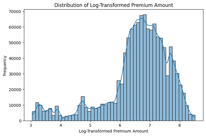
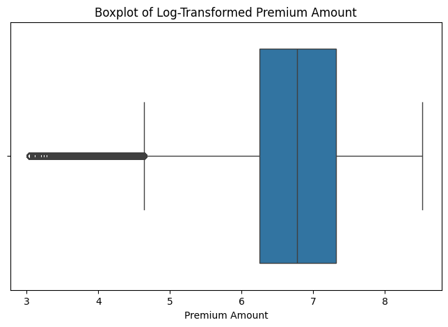
After the log transformation, the data is now closer to a normal (Gaussian-like) distribution.

5. Model Selection and Training

From the insights from the EDA step, we will use XGBoost for the best predictive model choice because it minimizes preprocessing needs while maximizing robustness and predictive performance.

• Handles missing values internally: No need to impute missing data manually — XGBoost learns the best path for missing values during tree splits.
• Robust to skewed numerical features: Tree-based models split data by thresholds, not by assuming normality (unlike linear models), so skewness is less of a problem.
• Supports raw categorical features (enable_categorical=True): Newer versions of XGBoost can handle categorical features directly, reducing the need for manual target encoding, label encoding, or one-hot encoding.
• Faster and better optimization: Using tree_method=’hist’, XGBoost optimizes faster, even for large datasets, and avoids overfitting by regularization.
• Better predictive performance: Especially in messy real-world datasets like insurance data, where you have mixed data types, missingness, and high skewness.
• LightGBM is faster but more sensitive to overfitting, especially on small leaves (leaf-wise split), and its categorical handling is less stable if many rare categories.
• The dataset (around 1.2M rows) is reasonably large but not massive (so XGBoost speed is fine).

Key Steps:

• Convert Categorical Columns: Set all categorical columns’ dtype to "category" (required for XGBoost’s enable_categorical=True to work properly).
• Define Features and Target: X = df without “Premium Amount”, y = "Premium Amount".
• Set up K-Fold Cross-Validation: Create a 5-fold CV splitter (KFold) to evaluate model stability across different subsets of data.
• Initialize Prediction Holders: oof_preds: Out-of-fold predictions (same size as X). feature_importance_df: Store feature importance for each fold.
• Loop Over Each Fold: For each fold (fold 1 to 5): Split Data into training and validation sets (X_train, X_valid, y_train, y_valid). Train XGBoost on training data and evaluate on validation data.
• Predict Validation Set (OOF Prediction): Predict X_valid and store predictions in the corresponding positions of oof_preds.
• Calculate Fold RMSLE: Calculate Root Mean Squared Log Error (RMSLE) for that fold and store.
• Store Feature Importance: Save feature importance values for each feature from the trained model for that fold in the corresponding positions of feature_importance_df.

# Convert Categorical Features to "category" dtype for XGBoost
for col in cat_features:
    df[col] = df[col].astype("category")

# Define Features and Target
X = df.drop(columns=["Premium Amount"])
y = df["Premium Amount"]

# Cross-Validation Setup (5-Fold)
kf = KFold(n_splits=5, shuffle=True, random_state=42)
oof_preds = np.zeros(len(X))  # Out-of-Fold Predictions
feature_importance_df = pd.DataFrame(index=X.columns)
rmsle_per_fold = []  # Store RMSLE per fold

# Train XGBoost with Cross-Validation
for fold, (train_idx, valid_idx) in enumerate(kf.split(X)):
    print(f"🚀 Training Fold {fold + 1}...")

    # Split Data
    X_train, X_valid = X.iloc[train_idx], X.iloc[valid_idx]
    y_train, y_valid = y.iloc[train_idx], y.iloc[valid_idx]

    # Train XGBoost Model with Native Categorical Handling
    model = XGBRegressor(
        enable_categorical=True,
        tree_method="hist",  # Optimized for speed
        max_depth=8,
        learning_rate=0.01,
        n_estimators=2000,
        colsample_bytree=0.9,
        subsample=0.9,
        early_stopping_rounds=50,
        eval_metric="rmse",
        random_state=42
    )
    model.fit(
        X_train, y_train,
        eval_set=[(X_valid, y_valid)],
        verbose=100
    )

    # Out-of-Fold Predictions
    fold_preds = model.predict(X_valid)
    oof_preds[valid_idx] = fold_preds

    # Calculate RMSLE for This Fold
    fold_rmsle = np.sqrt(mean_squared_log_error(np.expm1(y_valid), np.expm1(fold_preds)))
    rmsle_per_fold.append(fold_rmsle)
    print(f"✔ Fold {fold + 1} RMSLE: {fold_rmsle:.5f}")

    # Store Feature Importance
    feature_importance_df[f"Fold_{fold + 1}"] = model.feature_importances_

Output:

🚀 Training Fold 1...
[0]	validation_0-rmse:1.09602
[100]	validation_0-rmse:1.05936
[200]	validation_0-rmse:1.04985
[300]	validation_0-rmse:1.04745
[400]	validation_0-rmse:1.04674
[500]	validation_0-rmse:1.04652
[600]	validation_0-rmse:1.04640
[700]	validation_0-rmse:1.04635
[800]	validation_0-rmse:1.04631
[900]	validation_0-rmse:1.04630
[1000]	validation_0-rmse:1.04628
[1100]	validation_0-rmse:1.04628
[1116]	validation_0-rmse:1.04627
✔ Fold 1 RMSLE: 1.04627
🚀 Training Fold 2...
[0]	validation_0-rmse:1.09482
[100]	validation_0-rmse:1.05816
[200]	validation_0-rmse:1.04877
[300]	validation_0-rmse:1.04647
[400]	validation_0-rmse:1.04584
[500]	validation_0-rmse:1.04566
[600]	validation_0-rmse:1.04561
[700]	validation_0-rmse:1.04558
[771]	validation_0-rmse:1.04558
✔ Fold 2 RMSLE: 1.04557
🚀 Training Fold 3...
[0]	validation_0-rmse:1.09471
[100]	validation_0-rmse:1.05882
[200]	validation_0-rmse:1.04953
[300]	validation_0-rmse:1.04726
[400]	validation_0-rmse:1.04661
[500]	validation_0-rmse:1.04644
[600]	validation_0-rmse:1.04636
[700]	validation_0-rmse:1.04633
[800]	validation_0-rmse:1.04631
[900]	validation_0-rmse:1.04630
[950]	validation_0-rmse:1.04630
✔ Fold 3 RMSLE: 1.04630
🚀 Training Fold 4...
[0]	validation_0-rmse:1.09521
[100]	validation_0-rmse:1.05785
[200]	validation_0-rmse:1.04809
[300]	validation_0-rmse:1.04553
[400]	validation_0-rmse:1.04480
[500]	validation_0-rmse:1.04457
[600]	validation_0-rmse:1.04448
[700]	validation_0-rmse:1.04442
[800]	validation_0-rmse:1.04441
[900]	validation_0-rmse:1.04440
[1000]	validation_0-rmse:1.04438
[1100]	validation_0-rmse:1.04436
[1140]	validation_0-rmse:1.04438
✔ Fold 4 RMSLE: 1.04436
🚀 Training Fold 5...
[0]	validation_0-rmse:1.09641
[100]	validation_0-rmse:1.05924
[200]	validation_0-rmse:1.04941
[300]	validation_0-rmse:1.04689
[400]	validation_0-rmse:1.04616
[500]	validation_0-rmse:1.04592
[600]	validation_0-rmse:1.04583
[700]	validation_0-rmse:1.04577
[800]	validation_0-rmse:1.04574
[900]	validation_0-rmse:1.04572
[929]	validation_0-rmse:1.04572
✔ Fold 5 RMSLE: 1.04571

6. Model Evaluation

We evaluated models using:

• Root Mean Squared Log Error (RMSLE): Measures the average logarithmic difference between actual and predicted premium amounts, reducing the impact of large outliers and ensuring better performance on skewed data.
• Feature Importance Analysis: Identifies top factors influencing premium pricing.

# Compute and Print Overall RMSLE
overall_rmsle = np.mean(rmsle_per_fold)
print("\n📊 Cross-Validation RMSLE Scores per Fold:")
for i, score in enumerate(rmsle_per_fold):
    print(f"✔ Fold {i + 1} RMSLE: {score:.5f}")
print(f"\n🚀 Overall Cross-Validation RMSLE: {overall_rmsle:.5f}")

# Compute Final RMSLE Using All Out-of-Fold Predictions
final_rmsle = np.sqrt(mean_squared_log_error(np.expm1(y), np.expm1(oof_preds)))
print(f"\n✅ Final Model RMSLE: {final_rmsle:.5f}")

Output:

📊 Cross-Validation RMSLE Scores per Fold:
✔ Fold 1 RMSLE: 1.04627
✔ Fold 2 RMSLE: 1.04557
✔ Fold 3 RMSLE: 1.04630
✔ Fold 4 RMSLE: 1.04436
✔ Fold 5 RMSLE: 1.04571

🚀 Overall Cross-Validation RMSLE: 1.04564

✅ Final Model RMSLE: 1.04564

# Compute Average Feature Importance
feature_importance_df["Average"] = feature_importance_df.mean(axis=1)
feature_importance_df = feature_importance_df.sort_values(by="Average", ascending=False)

# Plot Top 20 Important Features
plt.figure(figsize=(12, 6))
sns.barplot(
    x=feature_importance_df["Average"][:20], 
    y=feature_importance_df.index[:20], 
    palette="viridis"
)
plt.xlabel("Feature Importance Score")
plt.ylabel("Features")
plt.title("Top 20 Important Features")
plt.show()

Output:

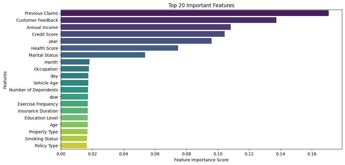
Key Actionable Insights:

• Previous Claims is the most influential factor in predicting premium amounts, indicating that individuals with past claims significantly impact the model’s predictions.
• Customer Feedback, Annual Income & Credit Score, highlighting the role of customer sentiment and financial stability in premium pricing.
• Year of policy start is among the top features, indicating a seasonal or yearly pattern in insurance premium pricing.
• Health Score plays a critical role, possibly due to its impact on risk assessment.
• Marital Status has moderate influence, likely because it somehow correlates with income stability and insurance needs.
• Since Previous Claims and Customer Feedback are the top predictors, collecting accurate and detailed historical claim data and customer feedback could enhance model performance.
• Since Annual Income, Credit Score, and Health Score play significant roles, insurers could offer targeted pricing based on these variables. This leads to a rising problem of segmenting customers based on financial & health data.
• The significance of year suggests that premiums might fluctuate seasonally, making it beneficial to explore time-series adjustments.

Next steps for improvements

To further enhance this insurance premium prediction project, the potential future steps are:

1. Build Scalable and Automated Data Pipelines:
   • Develop automated end-to-end pipelines by combining SQL for data extraction, Apache Airflow for scheduling and orchestration, and Databricks for collaborative data engineering and machine learning development at scale. (Focus: orchestrating and automating workflows across systems.)
2. Improve Project Structure and Maintainability
   • Use Kedro to structure the project into modular, reproducible, and maintainable pipelines. This ensures that as the project grows, it remains clean, easy to extend, and production-ready. (Focus: clean codebase design and reproducibility.)
3. Accelerate Large-Scale Data Processing and Modeling
   • Use Dask / RAPIDS to boost the speed of data processing and model training by using Dask for distributed parallel computing and RAPIDS for GPU-accelerated machine learning, enabling efficient handling of very large datasets. (Focus: computational performance and scalability.)
4. Productionize the Model with Containers and Cloud
   • Use Docker to package the model and its dependencies into a Docker container and deploy it on Kubernetes for scalable, reliable production serving.
   • Use Cloud Platforms (AWS, GCP, Azure) to deploy the solution in the cloud using services like AWS SageMaker, GCP Vertex AI, or Azure ML for robust training, deployment, and monitoring in production environments.
5. Further Enhancements for Model Quality and Reliability
   • Perform large-scale hyperparameter tuning using frameworks like Optuna or Ray Tune.
   • Add advanced model explainability using tools like SHAP or LIME to build stakeholder trust.
   • Set up real-time monitoring dashboards to track model drift, prediction quality, and data pipeline health over time.

Conclusion

This project successfully built a data-driven insurance premium prediction model using EDA, feature engineering, and XGBoost. Our model mimics the insurer’s pricing approach, revealing key premium factors while improving transparency.

The code of this project is available here.

For further inquiries or collaboration, please contact me at my email.