
A/B Testing with Highly-Skewed Data Using the Mann–Whitney U Test
When your data is highly skewed, traditional A/B tests like the t-test or z-test (see my previous posts P1 and P2) can give misleading results. These tests assume that data is normally distributed, or that the sample size is large enough for the Central Limit Theorem to smooth out the distribution.
But what if you’re comparing user spend, session times, or click counts, where a few large values dominate? In these cases, using the Mann–Whitney U (MWU) test can provide more robust and reliable results.
📌 What Is the Mann–Whitney U Test?
The MWU test (also known as the Wilcoxon rank-sum test) is a non-parametric test used to compare two independent groups. It does not assume normality and works by comparing the ranks of values instead of the values themselves.
✅ Key Features:
- Compares distributions, not means
- Robust to outliers and skewed data
- Tests whether one group tends to have larger values than the other
Workflow for A/B testing with MWU-Test
- Formulate Your Hypothesis
- Example: “Users who see Version B spend more time on the page than those who see Version A.”
- Check for Skew
- Plot histograms or use scipy.stats.skew().
- If data is heavily skewed, avoid the t-test.
- Use the Mann–Whitney U Test
- Convert values into ranks.
- Calculate the U Statistic from the ranks.
- Compute the z-score from the U Statistic
- Interpret the p-value
- Compute p-value from the computed z-score.
- A low p-value (e.g. < 0.05) suggests a statistically significant difference between groups.
Theory for A/B Testing with MWU-Test
🎯 Problem Setup
Suppose you’re testing a new landing page, and your metric of interest is the session duration between two versions of a landing page. You have:
- Group A (control): current landing page
- Group B (variant): new landing page
Suppose:
- \(X_1, X_2, \dots, X_{n_A}\) are the observed session durations in A
- \(Y_1, Y_2, \dots, Y_{n_B}\) are the observed session durations in B
🔍 Step 1: Define Hypotheses
The Mann–Whitney U test tests:
- Null hypothesis \(H_0\): there is no tendency for one group’s session durations to be systematically higher or lower than the other (i.e., they come from the same distribution), which is
or Group B tends to have larger values than Group A, i.e.,
\[H_0: P(X < Y) \leq 0.5, \,\, \text{(one-sided test)}\]- Alternative hypothesis \(H_1\): Variant B performs differently, i.e.,
or if B does not perform better, i.e.,
\[H_1: P(X < Y) > 0.5, \,\, \text{(one-sided test)}\]⚙️ Step 2: MWU Statistic Under \(H_0\)
The Mann–Whitney U statistic counts the number of times an observation from one group is less than or equal an observation from the other group:
\[U_A = \sum_{i=1}^{n_A} \sum_{j=1}^{n_B} \mathbb{I}_{(X_i < Y_j)} + 0.5 \sum_{i=1}^{n_A} \sum_{j=1}^{n_B} \mathbb{I}_{(X_i = Y_j)}\] \[U_B = \sum_{i=1}^{n_A} \sum_{j=1}^{n_B} \mathbb{I}_{(Y_j < X_i)} + 0.5 \sum_{i=1}^{n_A} \sum_{j=1}^{n_B} \mathbb{I}_{(Y_j = X_i)}\]where \(\mathbb{I}_{a} = 1\) if \(a\) is true, and \(\mathbb{I}_{a} = 0\), otherwise.
Computing \(U_A\) or \(U_B\) using the above definition requires \(n_A n_B\) comparison, which has time complexity of \(\mathcal{O}(n_A n_B)\) and becomes very expensive if the sample sizes are large.
Therefore, we will use a different way that is more computationally efficient using ranks of elements in both groups:
\[U_A = n_An_B + \frac{n_A (n_A+1)}{2} - R_A\] \[U_B = n_An_B + \frac{n_B (n_B+1)}{2} - R_B\]where \(R_A = \sum_{i=1}^{n_A} \text{rank}(X_i)\), \(R_B = \sum_{j=1}^{n_B} \text{rank}(Y_j)\) and \(\text{rank}(X_i)\) or \(\text{rank}(Y_j)\) is the rank of \(X_i\) or \(Y_j\) in the joint list of both groups A and B.
The explanation of the formula computing the \(U_A\) or \(U_B\) using ranks will be discussed at the end of this post.
Here, the step of “converting values into ranks” in the workflow can also reduce the influence of extreme values and enables the test to focus on the order of the data rather than the specific values.
🧮 Step 3: U-Statistic Under \(H_0\)
For large samples (typically \(n_A, n_B \geq 20\)), the central limit theorem (CLT) tells us that the U statistic is approximately normally distributed because \(U_A\) or \(U_B\) is the sum of \(n_An_B\) random variables.
The mean of \(U_A\) or \(U_B\) under \(H_0\) is
\[\mu_U = \frac{n_An_B}{2}\]The standard deviation of \(U_A\) or \(U_B\) under \(H_0\) is
\[\sigma_U = \sqrt{\frac{n_An_B}{12}(N+1 - T)}\]where \(N = n_A+n_B\) and
\[T = \frac{\sum_{i=1}^g (t_i^3-t_i)}{N(N-1)}\](These formulas come from the fact that, under the null hypothesis, every possible assignment of ranks is equally likely. This leads to a precise calculation of how the rank-sum varies. The detaild proof of these statistic parameters is out of the scope of this post.)
The z-score tells us how far the difference of the observed session duration we see is from zero, using standard error as the unit, assuming that \(H_0\) is true:
\[z = \frac{U-\mu_U}{\sigma_U}\]In practice, we often use \(U = \min(U_A,U_B)\) by convention to avoid confusion in one-sided tests.
However, mathematically, either \(U_A\) or \(U_B\) can be used as \(U\) and give the same z-score because they share the same mean and variance.
So,
- If \(z\) is close to 0, the observed difference is what we’d expect from random chance
- If \(z\) is far from 0, the difference is larger than what we’d expect from chance, so it might be statistically significant
📉 Step 4: Compute P-Value Under \(H_0\)
If the sample sizes are large, the steps of computing p-values based on the compuated z-score are similar to those in my previous post, and hence, omitted here.
If the sample sizes are small, we can calculate the p-value by using the exact distribution of \(U\), which takes into account the discrete nature of the test statistic rather than approximating it with a continuous normal distribution. We will not discuss this case in this post since the post is already too long.
Implementing an Example A/B Test in Python
Let’s simulate a basic A/B test for the session duration.
import numpy as np
from scipy.stats import mannwhitneyu
import matplotlib.pyplot as plt
# Simulated skewed data (e.g., log-normal)
np.random.seed(42)
group_A = np.random.lognormal(mean=2.0, sigma=1.0, size=100)
group_B = np.random.lognormal(mean=2.3, sigma=1.0, size=100)
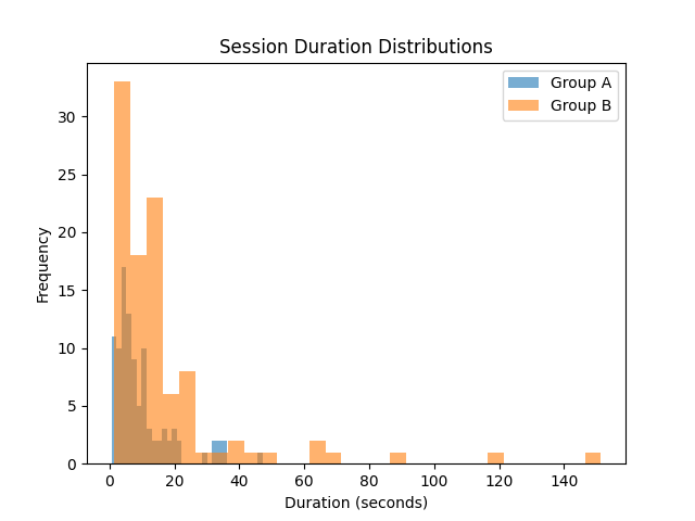
# Visualize the distributions
plt.hist(group_A, bins=30, alpha=0.6, label='Group A')
plt.hist(group_B, bins=30, alpha=0.6, label='Group B')
plt.legend()
plt.title("Session Duration Distributions")
plt.xlabel("Duration (seconds)")
plt.ylabel("Frequency")
plt.show()
# Run Mann–Whitney U test (two-sided)
stat, p = mannwhitneyu(group_A, group_B, alternative='less')
print(f"P-value: {p:.4f}")
Output:
P-value: 0.0023
With a p-value of 0.0023 significantly smaller than 0.05, we reject the null hypothesis and conclude that Group B performs significantly better.
Summary
The Mann–Whitney U test is a powerful and reliable method for A/B testing when your data is not normally distributed or is heavily skewed.
🚀 The code of the example is available here.
For further inquiries or collaboration, please contact me at my email.
Explanation for the Formula of Computing \(U_A\) or \(U_B\) using Ranks:
By definition of \(U_A\) and \(U_B\), the sum of \(U_A\) and \(U_B\) is the total number of comparisons, i.e.,
\[U_A + U_B = n_An_B\]If all \(X_i\) values were smaller than all \(Y_j\) values (i.e., the worst case), all these \(X_i\) would receive the lowest ranks: \(1,2,\dots,n_A\). Therefore, the minimum possible sum of ranks of group A is
\[R_{A,\min} = \sum_{i=1}^{n_A} \text{min rank of } X_i = \frac{n_A(n_A+1)}{2}\]Every time an \(X_i\) larger than \(Y_j\), the rank of \(X_i\) is pushed \(+1\) higher compared to its lowest ranks if it had lost that comparison.
Similarly, every time an \(X_i\) equals \(Y_j\), the rank of \(X_i\) is pushed \(+0.5\) higher compared to its lowest ranks if it had lost that comparison.
By these observations,
\[U_B = \sum_{i=1}^{n_A} \sum_{j=1}^{n_B} \mathbb{I}_{(Y_j < X_i)} + 0.5 \sum_{i=1}^{n_A} \sum_{j=1}^{n_B} \mathbb{I}_{(Y_j = X_i)} = R_A - R_{A,\min}\]which tells us how much the ranks of Group A exceed the “worst” scenario.
Now, since \(U_A + U_B = n_An_B\), we must have \(U_A = n_An_B - U_B = n_An_B + \frac{n_A (n_A+1)}{2} - R_A\). The derivation of \(U_B\) is similar to that of \(U_A\).