
The Ultimate Guide to A/B Testing: Workflow, Theory, and Python Example
A/B testing is a cornerstone of data-driven decision-making in product development, marketing, and user experience optimization. Whether you’re launching a new feature or redesigning a webpage, A/B testing helps you understand what works best for your users with scientific rigor.

🧪 What is A/B Testing?
A/B Testing, also known as split testing, is a controlled experiment comparing two versions (A and B) to determine which performs better for a specific outcome (e.g., clicks, conversions, or revenue).
Group A (the control) gets the original version.
Group B (the variant) gets the new version.
After collecting enough data, statistical analysis determines if one variant significantly outperforms the other.
Example:
You want to test if changing the color of a “Buy Now” button from blue to green increases purchases.
- Group A sees the blue button.
- Group B sees the green button.
You then measure the conversion rate in each group.
📈 Why is A/B Testing Important in Companies?
Companies rely on A/B testing to:
✅ Make data-driven decisions instead of relying on intuition
💰 Increase conversion rates and revenue
🔁 Continuously optimize user experience and features
📊 Measure the true impact of design or feature changes
🎯 Reduce risk by validating changes with a small user segment before full rollout
Industries like e-commerce, SaaS, gaming, and digital media use A/B testing extensively to fine-tune everything from email campaigns to checkout processes.
📝 Workflow for Conducting A/B Tests
1. Define the Objective
What metric do you want to improve? Examples: click-through rate, conversion rate, average revenue per user.
2. Form a Hypothesis
“Changing X will improve Y because Z.”
Example: “Changing the button color to green will increase the purchase rate because it stands out more.”
3. Split the Audience
Randomly assign users to:
- Group A (Control)
- Group B (Variant)
Ensure proper randomization and sample size.
4. Run the Experiment
Let the test run for a statistically valid time period. Avoid ending early due to random fluctuations.
5. Analyze the Results
Use statistical tests (e.g., t-test or z-test for proportions) to check for statistical significance.
6. Implement or Reject the Change
If the variant performs significantly better, consider deploying it to all users. If not, stick with the original.
Theory for A/B Testing
At its core, A/B testing is a statistical hypothesis test. It helps us determine whether the difference in performance between two groups (A and B) is statistically significant or due to random chance.
🎯 Problem Setup
Suppose:
- \(p_A\) is the true conversion rate in A
- \(p_B\) is the true conversion rate in B
These are unknown parameters we are trying to make inferences about using sample data:
- Group A (control) has \(n_A\) users with \(x_A\) conversions
- Group B (variant) has \(n_B\) users with \(x_B\) conversions
Then:
- \(\hat{p}_A = \frac{x_A}{n_A}\) is the observed conversion rate in A
- \(\hat{p}_B = \frac{x_A}{n_B}\) is the observed conversion rate in B
We use \(\hat{p}_A\) and \(\hat{p}_B\) to estimate \(p_A\) and \(p_B\). We also use hypothesis testing to decide if the difference in the observed conversion rates is statistically significant.
🔍 Step 1: Define Hypotheses
- Null hypothesis \(H_0\): No difference in conversion rates, i.e.,
- Alternative hypothesis \(H_1\): Variant B performs differently, i.e.,
or if B is better, i.e.,
\[H_1: p_B > p_A \,\, \text{(one-sided test)}\]📊 Step 2: Pooled Conversion Rate Under \(H_0\)
Assume \(H_0\) is true, the true conversion rates are equal to \(p\), i.e., \(p_A = p_B = p\). We treat both groups as coming from the same population. Since \(p\) is usually unknown in real-world tests, we compute the pooled estimate of \(p\) instead:
\[\hat{p} = \frac{x_A+x_B}{n_A+n_B}\]⚙️ Step 3: Estimated Standard Error (SE) Under \(H_0\)
SE is a measure of the uncertainty or variability in the difference between two observed conversion rates \(\hat{p}_A\) and \(\hat{p}_B\). It tells you how much the observed difference between groups A and B might vary just due to random sampling.
In simple terms, SE tells you how much “wiggle room” you should expect in your A/B test results — even if there were actually no real difference in the true conversion rates of A and B.
The true SE for the difference in the observed conversion rates under \(H_0\) is:
\[\text{SE} = \sqrt{p(1 - p)\Big(\frac{1}{n_A} + \frac{1}{n_B}\Big)}\](This expression will be explained at the end of the post)
However, this true SE is only theoretical because \(p\) is unknown.
Instead, the estimated SE for the difference in the observed conversion rates is computed using the estimate \(\hat{p}\) of \(p\):
\[\text{SE} = \sqrt{\hat{p}(1 - \hat{p})\Big(\frac{1}{n_A} + \frac{1}{n_B}\Big)}\]🧮 Step 4: Z-Statistic Under \(H_0\)
The z-score tells us how far the difference of the observed conversion rates we see is from zero, using standard error as the unit, assuming that \(H_0\) is true:
\[z = \frac{\hat{p}_B - \hat{p}_A}{\text{SE}}\]So,
- If \(z\) is close to 0, the observed difference is what we’d expect from random chance
- If \(z\) is far from 0, the difference is larger than what we’d expect from chance, so it might be statistically significant
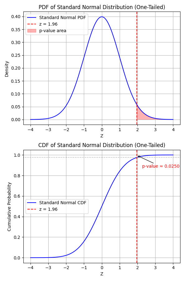
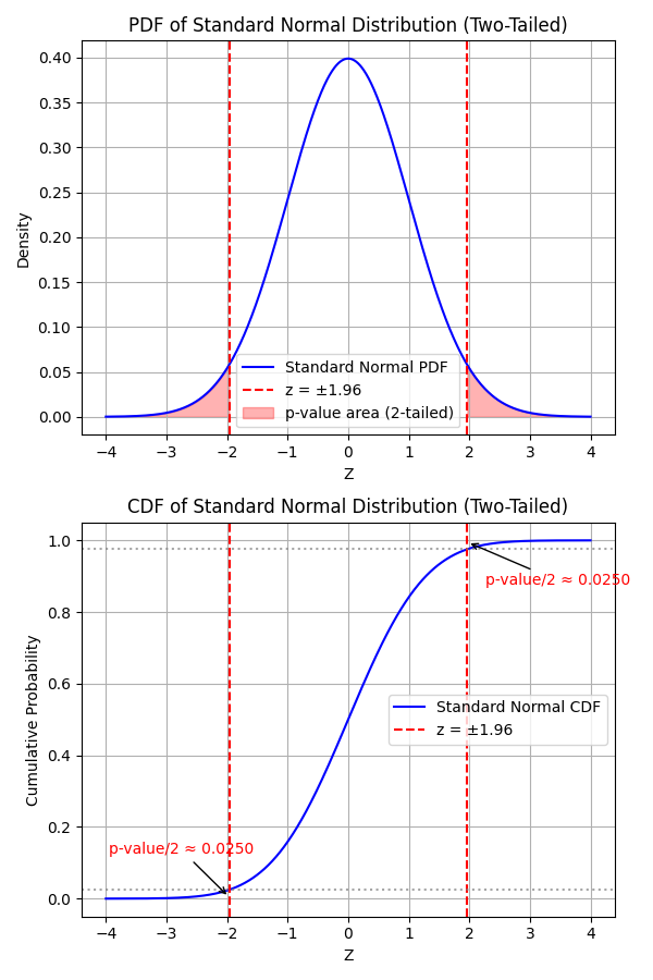
📉 Step 5: Compute P-Value Under \(H_0\)
Just knowing “how many standard errors away” from the computed z-score is isn’t enough — we want to quantify how likely it is to observe such a result by chance.
To do this, given the z-score formula above, we transform it into the standard normal scale — a distribution with: Mean = 0, Standard deviation = 1, Symmetrical bell shape.
If the sample size is large, the Central Limit Theorem tells us that the difference \(\hat{p}_B - \hat{p}_A\) (appropriately normalized) follows an approximately normal distribution — so the z-score follows the standard normal distribution (i.e., z-distribution).
We use the z-score to find a p-value from the standard normal distribution.
The p-value answers this question: “If the null hypothesis \(H_0\) is true, what is the probability of seeing a result this extreme or more extreme just by chance?”
Mathematically, p-value is the area under the curve of the standard normal distribution beyond your z-score.
- For a two-tailed test:
- For a one-tailed test:
where \(\Phi (z)\) is the cumulative distribution function (CDF) of the standard normal distribution.
Example: Say your z-score is 1.96. Using the standard normal table:
- For one-tailed test, \(p_{value} = P(Z > 1.96) = 1 - \Phi (1.96) = 0.025\)
- For a two-tailed test, \(p_{value} = 2 P(Z > 1.96) = 0.05\)
So there’s a \(5\%\) chance you’d observe such a difference (or bigger) if there really were no true difference.
✅ Step 6: Decide to reject \(H_0\) or not
- If \(p_{value} < \alpha\) (commonly \(0.05\)), we reject \(H_0\) and conclude that the difference is statistically significant.
- Otherwise, we fail to reject \(H_0\).
Implementing an Example A/B Test in Python
Let’s simulate a basic A/B test for conversion rates.
import numpy as np
import scipy.stats as stats

# Simulated data
# Group A (Control): 1000 users, 120 conversions
# Group B (Variant): 1000 users, 138 conversions

control_conversions = 120
variant_conversions = 138
control_total = 1000
variant_total = 1000

# Conversion rates
p1 = control_conversions / control_total
p2 = variant_conversions / variant_total
p_pooled = (control_conversions + variant_conversions) / (control_total + variant_total)

# Standard error
se = np.sqrt(p_pooled * (1 - p_pooled) * (1/control_total + 1/variant_total))

# z-score
z = (p2 - p1) / se

# p-value
p_val = 1 - stats.norm.cdf(z)

print(f"Control conversion rate: {p1:.2%}")
print(f"Variant conversion rate: {p2:.2%}")
print(f"Z-score: {z:.4f}")
print(f"P-value: {p_val:.4f}")
Output:
Control conversion rate: 12.00%
Variant conversion rate: 13.80%
Z-score: 1.2008
P-value: 0.1149
Since the p-value is ~0.1149, it’s significantly above the typical 0.05 threshold. We fail to reject \(H_0\), which means the improvement is not statistically significant.
⚠️ Common Pitfalls and Best Practices
❌ Pitfalls
- Stopping tests too early: Can lead to false positives.
- Multiple testing without correction: Increases false discovery rates.
- Non-random assignment: Biases results.
- Too small sample size: Leads to underpowered tests.
- Ignoring external factors: Holidays, promotions, etc., may skew results.
✅ Best Practices
- Pre-calculate required sample size and test duration.
- Randomize users consistently (not on each visit).
- Use server-side experiments for better control.
- Run tests long enough to capture variability (typically 1-2 weeks).
- Segment results by key user dimensions (device type, location, etc.).
- Apply corrections when running multiple simultaneous tests (e.g., Bonferroni).
Summary
A/B testing is a powerful yet simple tool that enables product and marketing teams to experiment with confidence. By following a structured approach and avoiding common pitfalls, companies can harness A/B testing to drive measurable growth and make smarter decisions.
🚀 The code of the example is available here.
For further inquiries or collaboration, please contact me at my email.
Expression of SE Explained:
SE is the standard error of \(\hat{p}_B - \hat{p}_A\), i.e., \(\text{SE} = \sqrt{\text{Var} (\hat{p}_B - \hat{p}_A)}\)
Recall that under \(H_0\), both groups A and B has the same conversion rate \(p\). Without loss of generality, consider group A with \(n_A\) trials (e.g., show a button to users). Each trial \(i\) is a Bernoulli random variable \(X_i \in \{0,1\}\), in which the probability of \(X_i=1\) (conversion) is \(p\), i.e., \(X_i \sim \text{Bernoulli} (p)\). Then,
\[\mathbb{E}(X_i) = p\] \[\text{Var}(X_i) = \mathbb{E}(X_i^2) - (\mathbb{E}(X_i))^2 = p\times 1^2 + (1-p)\times 0^2 - p^2 = p(1-p)\] \[x_A = \sum_{i=1}^{n_A} X_i\]Therefore, by definition of the Binomial distribution, \(x_A \sim \text{Binomial} (n_A, p)\).
Then, \(\mathbb{E}(x_A) = n_A p\) and \(\mathbb{E}(\hat{p}_A) = \mathbb{E}( \frac{x_A}{n_A} ) = \frac{1}{n_A} \mathbb{E}( x_A ) = \frac{n_A p }{n_A} = p\) — the true popolation conversion rate. This means \(\hat{p}_A\) an biased estimator of \(p\).
\[\text{Var}(x_A) = \sum_{i=1}^{n_A} \text{Var}(X_i) = n_A p (1-p)\] \[\text{Var}(\hat{p}_A) = \text{Var}\Big(\frac{x_A}{n_A}\Big) = \frac{\text{Var}(x_A)}{n_A^2} = \frac{n_A p (1-p)}{n_A^2} = \frac{p (1-p)}{n_A}\]Central Limit Theorem (CLT) allows us to treat the distribution of \(\hat{p}_A\) as an approximate normal distribution for a large population, i.e., \(\hat{p}_A \sim \text{Approximately Normal} \Big(p, \frac{p(1-p)}{n_A}\Big)\).
Now, consider both \(\hat{p}_A\) and \(\hat{p}_B\). Since these variables are independent, their varience is
\(\text{Var} (\hat{p}_B - \hat{p}_A) = \text{Var} (\hat{p}_B) + \text{Var} (\hat{p}_A) = p(1-p)\Big(\frac{1}{n_A}+\frac{1}{n_B}\Big)\).
Then, the expression of SE is obtained via \(\text{SE} = \sqrt{\text{Var} (\hat{p}_B - \hat{p}_A)}\).